Chapter 9 Disease-spatial patterns
This chapter contains an introduction to different types of spatial data, the theory of spatial lattice processes and introduces disease mapping and models for performing smoothing of risks over space. The reader will have gained an understanding of the following topics:
disease mapping and how to improve estimates of risk by borrowing strength from adjacent regions which can reduce the instability inherent in risk estimates based on small (expected) numbers;
- how smoothing can be performed using either the empirical Bayes or fully Bayesian approaches;
- computational methods for handling areal data;
- Besag’s seminal contributions to the field of spatial statistics including the very important concept of a Markov random field;
- approaches to modelling areal data including conditional autoregressive models;
- how Bayesian spatial models for lattice data can be fit using NIMBLE, RStan and R–INLA.
Example 9.1: Empirical Bayes and Bayes smoothing of COPD mortality for 2010
Here we consider hospitalization for a respiratory condition, chronic obstructive pulmonary disease (COPD), in England in 2010. There are \(N_l=324\) local authority administrative areas each with an observed, \(Y_l\) and expected, \(E_l\), number of cases, \(l=1,...,324\). As described in
Section 2.4 the expected numbers were calculated using indirect standardization by applying the
age–sex specific rates for the whole of England to the age–sex population profile of each of the areas. In order to perform empirical Bayes smoothing, we will use the eBayes function in the SpatialEpi package.
This example uses the englandlocalauthority.shp, copdmortalityobserved.csv, and
copdmortalityexpected.csv datasets.
9.0.1 Empirical Bayes estimate using SpatialEpi
# requires SpatialEpi package
library (SpatialEpi)
library(sf) # package used to read shapefiles
# Laoding the borders of England
england <- read_sf("data/copd/englandlocalauthority.shp")
# Loading the data
observed <-
  read.csv(file = "data/copd/copdmortalityobserved.csv", row.names = 1)
expected <-
  read.csv(file = "data/copd/copdmortalityexpected.csv", row.names = 1)
#observed data
Y <- observed$Y2010
# offset
E <- expected$E2010

RRs = eBayes (Y , E )
plot ( RRs $ SMR , RRs $ RR , xlim = c (0 ,2) , ylim = c (0 ,2) , xlab = "
SMRs " , ylab = " RRs " )
abline ( a =0 , b =1 , col = " red " , lwd =3)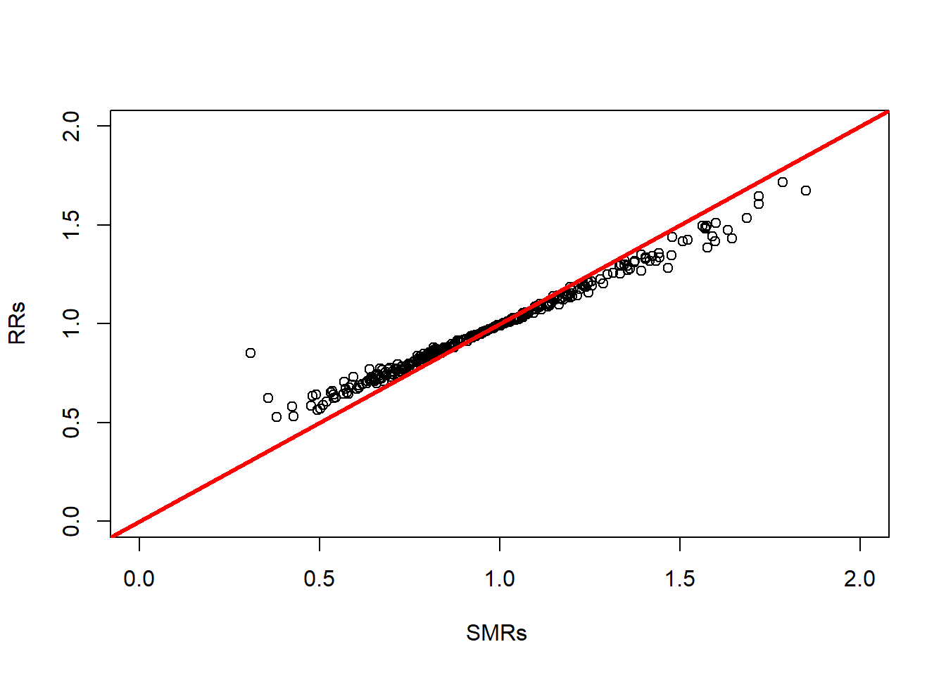
The smoothing can be seen with lower and higher SMRs being brought close to the overall average, \(\mu\) which in this case is \(\exp(-0.0309) = 0.9696\). Note that in this example, the areas are relatively large and would be expected to have substantial populations, so the effect of the smoothing is limited. In this example, \(\alpha\) was estimated to be 14.6. For a fully Bayesian, rather than empirical Bayes, analysis we can use NIMBLE; and this is what we present next.
Nimble
library(nimble)


Example9_1Nimble <- nimbleCode({
  for (i in 1:N) {
    Y[i] ~ dpois(mu[i])
    # REVIEW: There is an intercept in the book,
    # but then we wouldn't be able to compare it to example 5.2
    mu[i] <- E[i]*exp(beta0)* theta[i]
    #mu[i] <- E[i]* theta[i]
    # REVIEW: Same as before, the example in the book has theta[i] ~ Ga(a,a)
    theta[i] ~ dgamma(a, a)
    Y.fit[i] ~ dpois(mu[i])
  }
  # Priors
  a ~ dgamma(1,1)
  beta0 ~ dnorm(0, 10)

})

# Define the constants, data and initials lists for the `nimble` model.

# observations
y <- observed$Y2010
# offset
E <- expected$E2010
N <- length(y)
# constants list
constants <- list(
  N = N,
  E = E
)
# data list
ex.data <- list(Y = y)
# initial values list
inits <-
    list(
      theta = rgamma(N, 1, 1),
      a = rgamma(1, 1),
      beta0 = 0,
      Y.fit = rpois(N, E)
    )
# parameters to monitor
params <- c("theta", "a", "beta0", "Y.fit")

# Run model in nimble
mcmc.out <- nimbleMCMC(
  code = Example9_1Nimble,
  constants = constants,
  data = ex.data,
  inits = inits,
  monitors = params,
  niter = 50000,
  nburnin = 20000,
  thin = 14,
  WAIC = TRUE,
  nchains = 2,
  summary = TRUE,
  samplesAsCodaMCMC = TRUE
)
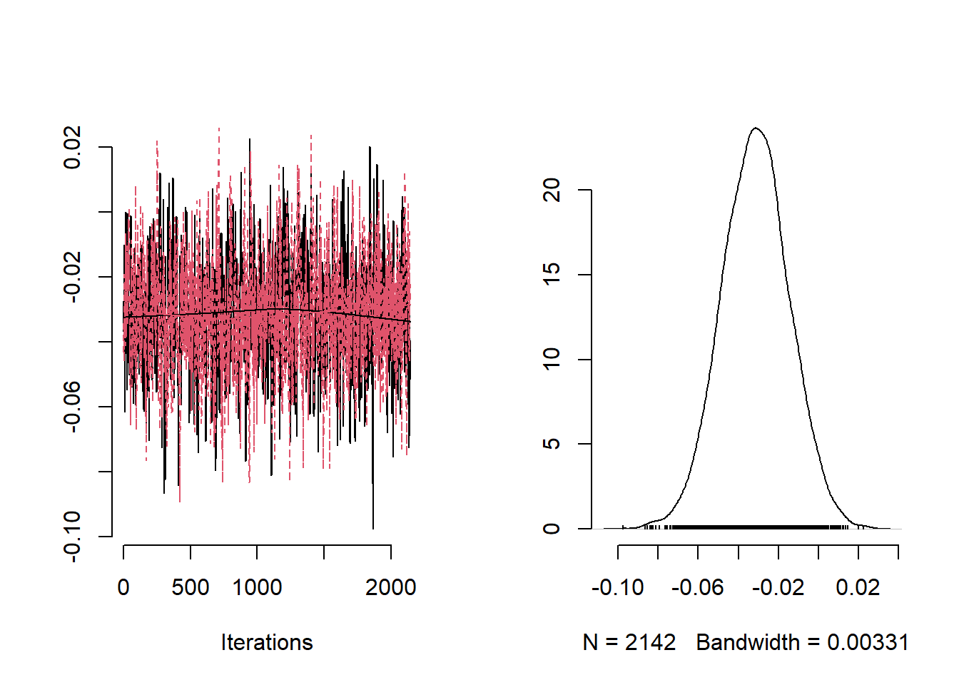
Effective sample size is checked through the minimum value among all the samples available. This is to check if this minimum is acceptable. We also provide trace plots of the chains for some of the parameters. We provide the command to obtain WAIC in case model comparison will be performed in a later stage.
## [1] 948.4589## nimbleList object of type waicList
## Field "WAIC":
## [1] 2422.992
## Field "lppd":
## [1] -1061.364
## Field "pWAIC":
## [1] 150.132#storing the samples from the posterior distribution in mvSamples
mvSamples <- mcmc.out$samples
# trace plot of a
plot(mvSamples[, c("a")], bty = "n")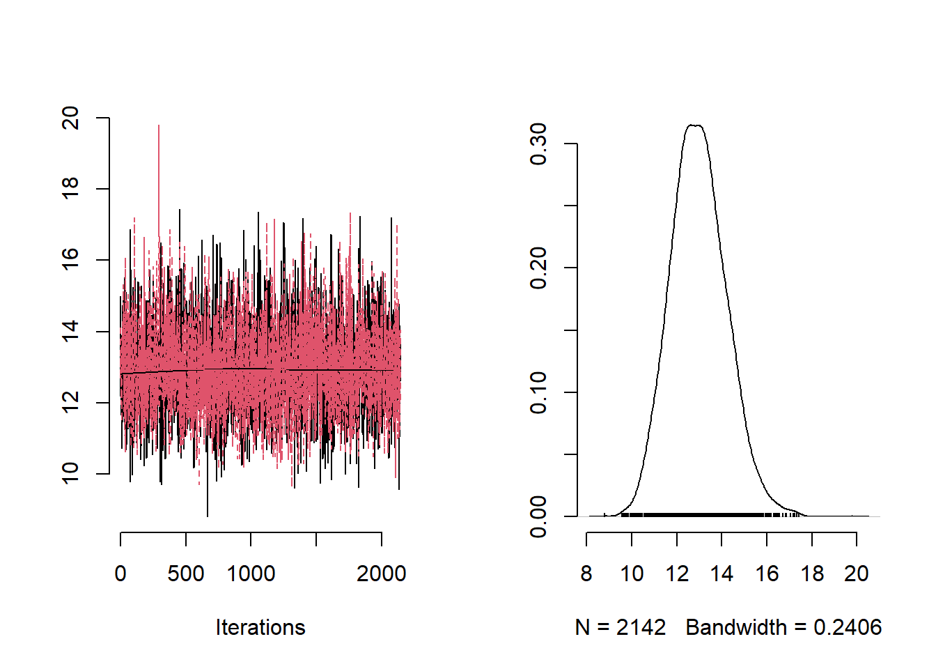
# trace plots of theta
for (i in 1:3)
  plot(mvSamples[, c(paste("theta[", i, "]", sep = ""))], bty = "n")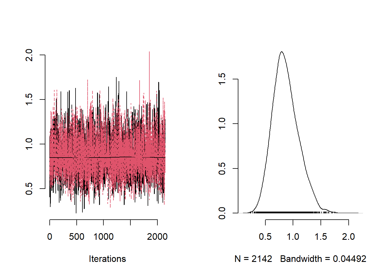
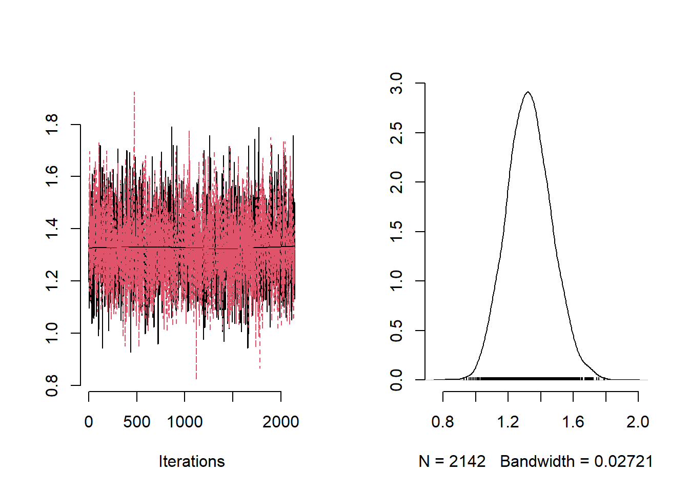
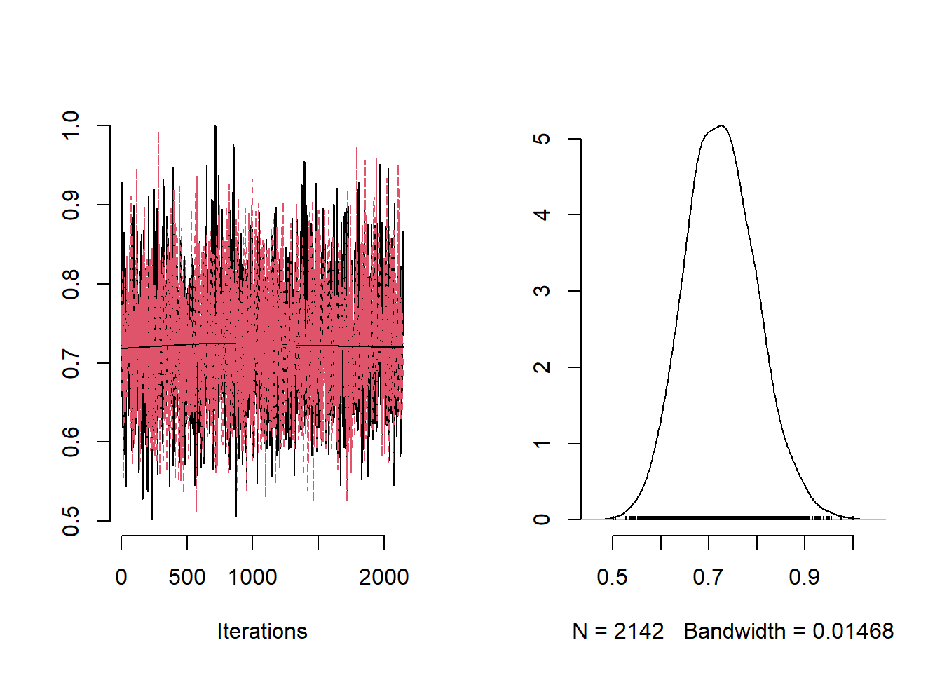
Now that we have checked the convergence of the chains we can plot the posterior mean and 95% CIs for each of the parameters.
##
## Iterations = 1:2142
## Thinning interval = 1
## Number of chains = 2
## Sample size per chain = 2142
##
## 1. Empirical mean and standard deviation for each variable,
##    plus standard error of the mean:
##
##           Mean      SD  Naive SE Time-series SE
## a     12.97734 1.23282 0.0188354      0.0193663
## beta0 -0.03137 0.01673 0.0002556      0.0005469
##
## 2. Quantiles for each variable:
##
##          2.5%     25%      50%      75%     97.5%
## a     10.7242 12.1384 12.92600 13.75815 15.546804
## beta0 -0.0642 -0.0427 -0.03132 -0.02042  0.001347
# posterior summaries of theta_i
post_summary <- mcmc.out$summary$all.chains |> as.data.frame() |>
tibble::rownames_to_column("variable")
# plot the mean and 95% CIs for the thetas
post_theta <-
post_summary[grepl("theta\\[", post_summary$variable),]
par(mfrow = c(1, 1))
plot(
post_theta$Mean,
pch = 19,
cex = 0.8,
bty = "n",
xlab = "Borough",
ylab = "Posterior Summary Rate",
ylim = c(min(post_theta$`95%CI_low`), max(post_theta$`95%CI_upp`))
)
for (i in 1:N)
segments(i, post_theta$`95%CI_low`[i], i, post_theta$`95%CI_upp`[i])
abline(h = 1, lwd = 2, lty = 2)
# posterior summary of fitted values
post_fitted <-
  post_summary[grepl("Y.fit\\[", post_summary$variable),]
# plot mean and 95% CIs for the fitted values
par(mfrow = c(1, 1))
plot(
  y,
  post_fitted$Mean,
  ylim = c(min(post_fitted$`95%CI_low`), max(post_fitted$`95%CI_upp`)),
  xlab = "Observed",
  ylab = "Fitted",
  pch = 19,
  cex = 0.7,
  bty = "n"
)
for (i in 1:N)
  segments(y[i], post_fitted$`95%CI_low`[i], y[i], post_fitted$`95%CI_upp`[i])
abline(a = 0, b = 1)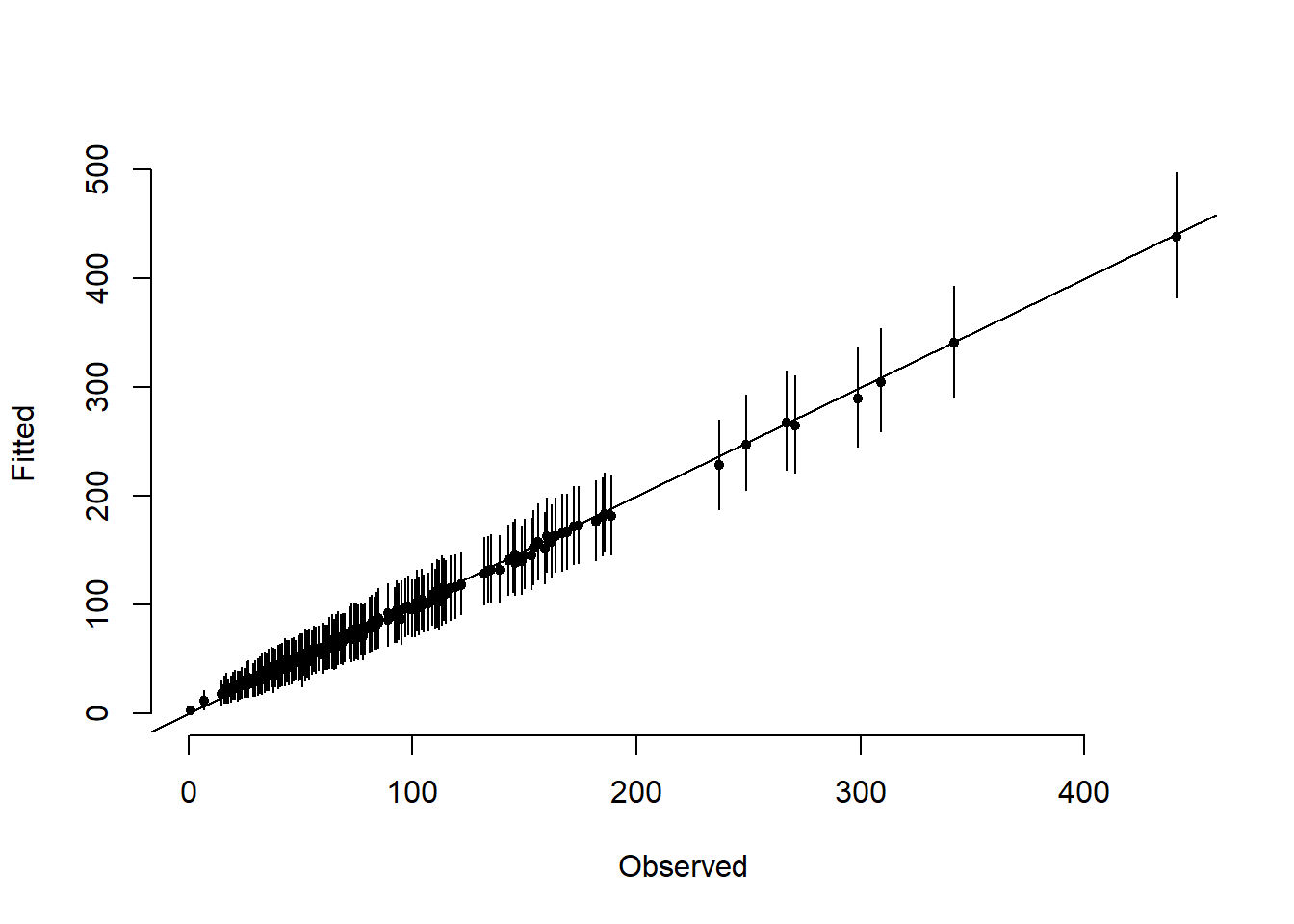
Now we present the code for the same model in {}. We start by cleaning the ´R environment`.
Stan
library(rstan)
library(sf) # to read shapefile
library(loo) # To calculate WAIC
options(mc.cores = parallel::detectCores())
rstan_options(auto_write = TRUE)

# Load data
# Reading in borders
england <- read_sf("data/copd/englandlocalauthority.shp")
# Reading in data
observed <-
  read.csv(file = "data/copd/copdmortalityobserved.csv", row.names = 1)
expected <-
  read.csv(file = "data/copd/copdmortalityexpected.csv", row.names = 1)
The Stan model is in a separate file called Example9_1.stan that will be called later.
data {
  int<lower=0> N;
  real<lower=0> E[N]; // need to indicate that variable is strictly positive
  int<lower=0> Y[N];
}

parameters {
  real<lower=0> theta[N];
  real<lower=0> a;
  real beta0;
}

transformed parameters{
  real <lower=0> mu[N];

  for(i in 1:N){
    mu[i]=E[i]*theta[i]*exp(beta0);
  }

}

model {
  // likelihood function and prior for theta
  for(i in 1:N){
    Y[i] ~ poisson(mu[i]);
    theta[i]~gamma(a,a);
  }
  a~gamma(1, 1);
  beta0~normal(0,10);
}

generated quantities {
  vector [N] log_lik;
  int<lower=0> yfit [N];

  //computing the log_likelihood for each value of the mean mu and the fitted values
  for(i in 1:N){
    log_lik[i]=poisson_lpmf(Y[i] |mu[i]);
    yfit[i]=poisson_rng(mu[i]);
  }

}
Similarly to NIMBLE, we now define the different objects that will contain information about the data.
# observations
y <- observed$Y2010
# offset
E <- expected$E2010
N <- length(y)
# data list
ex.data <- list(
  N = length(y),
  Y = y,
  E = E
)
# Run the model in Stan
Ex9_1Stan <- stan(
  file = "functions/Example9_1.stan",
  data = ex.data,
  chains = 3,
  iter = 10000,
  warmup = 3000,
  thin = 14,
  # QUESTION: should we explain this?
  control = list(adapt_delta = 0.8, max_treedepth = 15),
  init = "random",
  pars = c("a","beta0","theta", "log_lik", "yfit"),
  include = TRUE
)
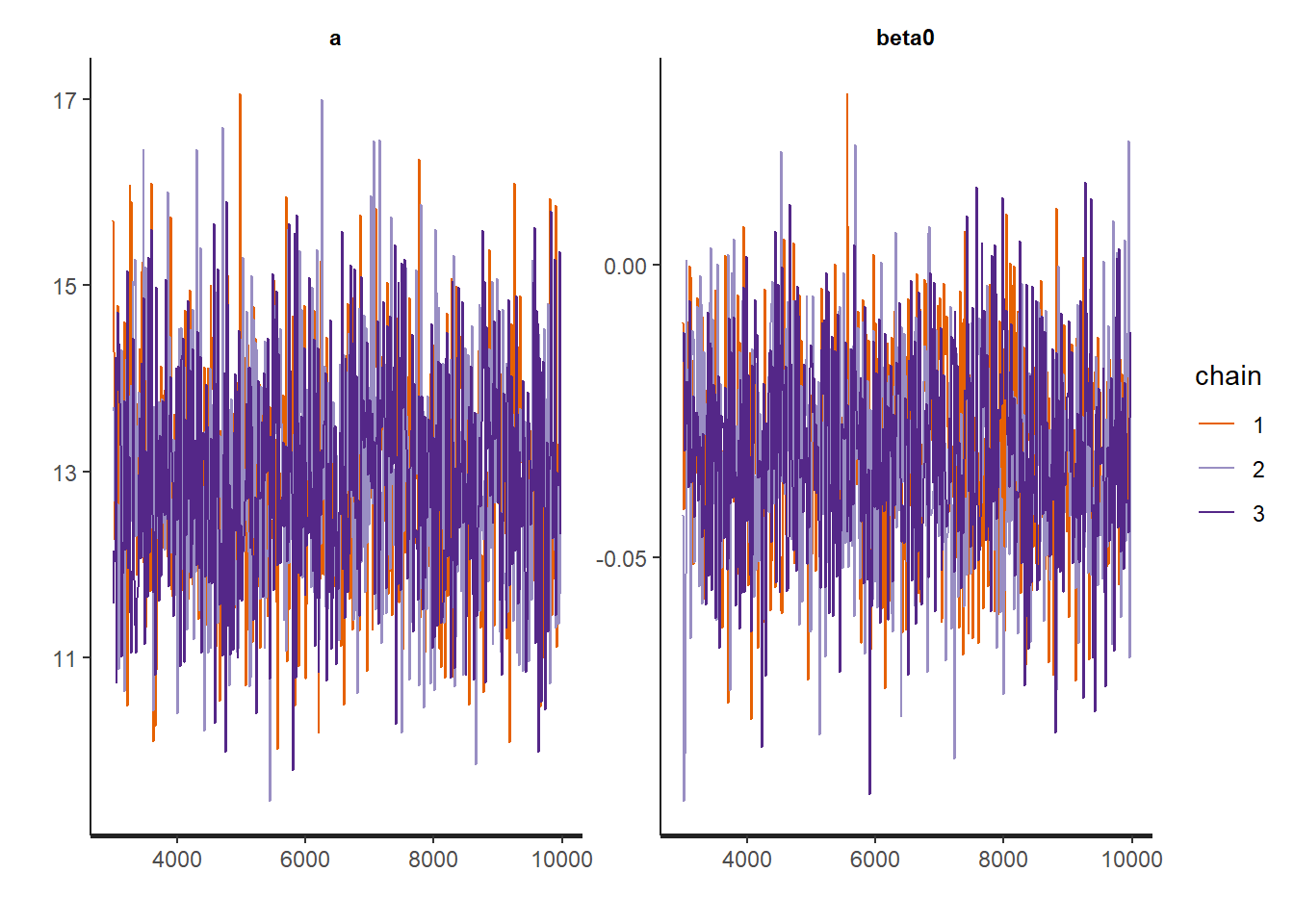
We now check the trace plots of some of the parameters, check the effective sample size. Once convergence has been checked we obtain the posterior summaries of some of the parameters.
# traceplots of parameter theta
rstan::traceplot(Ex9_1Stan, pars = c("theta[1]", "theta[2]", "theta[3]"))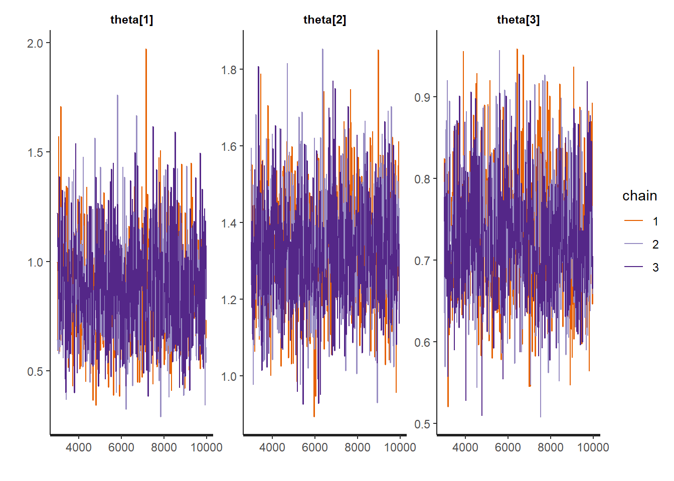
# posterior summaries together with Rhat
rstan::traceplot(Ex9_1Stan, pars = c("a","theta[1]", "theta[2]", "theta[3]"))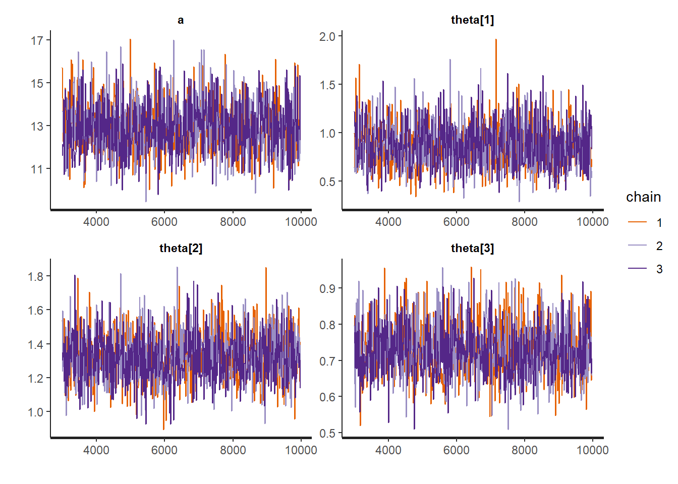
## $summary
##                mean     se_mean         sd       2.5%        25%        50%
## a        12.9490131 0.030133132 1.21097052 10.7279153 12.1160782 12.8953865
## theta[1]  0.8681535 0.005872796 0.22967964  0.4789593  0.6960057  0.8597968
## theta[2]  1.3269027 0.004045516 0.14569941  1.0538612  1.2254400  1.3209029
## theta[3]  0.7293979 0.002208173 0.07439276  0.5962105  0.6774943  0.7211274
##                75%      97.5%    n_eff      Rhat
## a        13.729623 15.3851313 1615.023 0.9998414
## theta[1]  1.016351  1.3539740 1529.520 0.9999455
## theta[2]  1.419336  1.6207442 1297.083 1.0004835
## theta[3]  0.777150  0.8885225 1134.998 1.0007149
##
## $c_summary
## , , chains = chain:1
##
##           stats
## parameter        mean         sd       2.5%        25%        50%        75%
##   a        12.9391260 1.20688131 10.6647963 12.1367051 12.8610229 13.7066434
##   theta[1]  0.8544009 0.21847768  0.4610477  0.7025649  0.8516174  0.9842713
##   theta[2]  1.3309053 0.14915119  1.0589718  1.2319590  1.3220494  1.4277758
##   theta[3]  0.7328573 0.07826966  0.5966028  0.6769945  0.7249705  0.7835412
##           stats
## parameter       97.5%
##   a        15.5179697
##   theta[1]  1.3197144
##   theta[2]  1.6162752
##   theta[3]  0.8917676
##
## , , chains = chain:2
##
##           stats
## parameter        mean         sd       2.5%        25%        50%        75%
##   a        12.9631607 1.23242884 10.7069049 12.1322796 12.9113706 13.7432376
##   theta[1]  0.8706192 0.23177021  0.4891381  0.6946233  0.8573132  1.0206591
##   theta[2]  1.3338165 0.14394937  1.0460653  1.2392597  1.3249056  1.4239841
##   theta[3]  0.7297883 0.07502032  0.5907728  0.6779665  0.7205219  0.7788053
##           stats
## parameter       97.5%
##   a        15.3983920
##   theta[1]  1.3767840
##   theta[2]  1.6308883
##   theta[3]  0.8904337
##
## , , chains = chain:3
##
##           stats
## parameter        mean         sd       2.5%        25%        50%        75%
##   a        12.9447526 1.19560290 10.7837245 12.0674517 12.9678053 13.7452054
##   theta[1]  0.8794403 0.23811021  0.4884869  0.6921386  0.8671821  1.0340745
##   theta[2]  1.3159863 0.14359380  1.0602166  1.2078908  1.3137105  1.4073229
##   theta[3]  0.7255480 0.06959774  0.6008815  0.6771501  0.7190926  0.7718208
##           stats
## parameter       97.5%
##   a        15.2901383
##   theta[1]  1.3849875
##   theta[2]  1.6040231
##   theta[3]  0.8703692
# To be able to compute the WAIC in Stan, we need to define the log_lik quantity in the generated quantities block
# Compute WAIC
loglik0 <- extract_log_lik(Ex9_1Stan)
waic0 <- waic(loglik0)
waic0##
## Computed from 1500 by 324 log-likelihood matrix
##
## Estimate SE
## elpd_waic -1210.4 8.0
## p_waic 149.3 3.9
## waic 2420.8 16.0
##
## 176 (54.3%) p_waic estimates greater than 0.4. We recommend trying loo instead.Note that the ´summaryfunction of aRStan` object provides the effective sample size and Rhat. We now plot the posterior summaries of \(\theta_i\) and each of the fitted values with their respective 95% posterior credible intervals.
summary_theta <-
  summary(Ex9_1Stan,
          pars = c("theta"),
          probs = c(0.05, 0.95))$summary |> as.data.frame()

par(mfrow = c(1, 1))
plot(
  summary_theta$mean,
  pch = 19,
  cex = 0.8,
  bty = "n",
  xlab = "Borough",
  ylab = "Posterior Summary Rate",
  ylim = c(min(summary_theta$`5%`), max(summary_theta$`95%`))
)
for (i in 1:N)
  segments(i, summary_theta$`5%`[i], i, summary_theta$`95%`[i])
abline(h = 1, lwd = 2, lty = 2)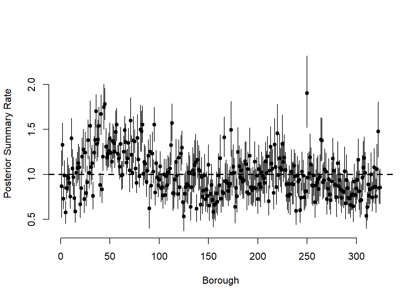
# Posterior summary of fitted values
summary_fit <-
  summary(Ex9_1Stan,
          pars = c("yfit"),
          probs = c(0.05, 0.95))$summary |> as.data.frame()
# Plot mean and 95% CIs for the fitted values
par(mfrow = c(1, 1))
plot(
  y,
  summary_fit$mean,
  ylim = c(min(summary_fit$`5%`), max(summary_fit$`95%`)),
  xlab = "Observed",
  ylab = "Fitted",
  pch = 19,
  cex = 0.7,
  bty = "n"
)
for (i in 1:N)
  segments(y[i], summary_fit$`5%`[i], y[i], summary_fit$`95%`[i])
abline(a = 0, b = 1)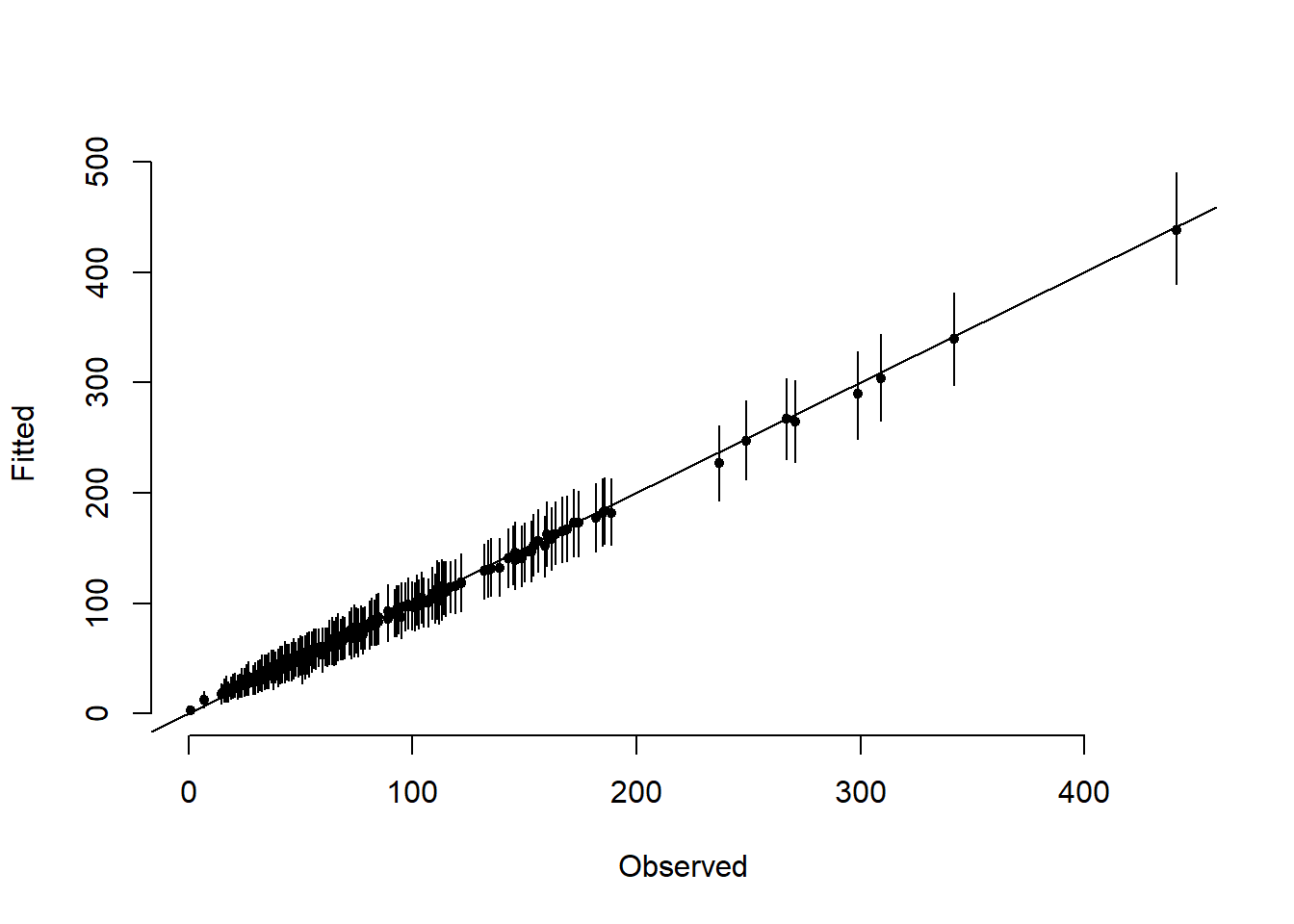
Example 9.3: Fitting a conditional spatial model in NIMBLE and RStan
In this example, we see how to fit the Poisson log–normal model seen in Section 9.4 with spatial random effects coming from the ICAR model described in Section 9.3.1.
This example uses the englandlocalauthority.shp, copdmortalityobserved.csv, and copdmortalityexpected.csv datasets.
Nimble
In this example, we see how to fit the Poisson log–normal model seen in Section 9.4 with spatial random effects coming from the ICAR model described in Section 9.3.1.
We start by loading some packages and the data.
library(ggplot2) # to plot map
library(spdep) # read the shapefile (read_sf) and build neighbors list (poly2nb)
library(nimble)

# Load data
# Reading in borders
england <- read_sf("data/copd/englandlocalauthority.shp")
# Reading in data
observed <-
  read.csv(file = "data/copd/copdmortalityobserved.csv", row.names = 1)
expected <-
  read.csv(file = "data/copd/copdmortalityexpected.csv")
covariates <- read.csv(file = "data/copd/copdavgscore.csv")
# Merge everything into one data frame
copd_df <-
  cbind(observed,  expected) |> merge(
    covariates,
    by.x = "code",
    by.y = "LA.CODE",
    all.x = TRUE,
    all.y = FALSE
  )
The following command provides a scatter plot of the average deprivation score and the estimated SMR for 2010. The plot suggests that as deprivation increases so does the SMR for 2010.
copd_df$SMR2010 = copd_df$Y2010 / copd_df$E2010

ggplot(copd_df) + geom_point(aes(x = Average.Score, y = SMR2010)) +
  theme_classic() + ylab("SMR 2010") + xlab("Average deprivation score")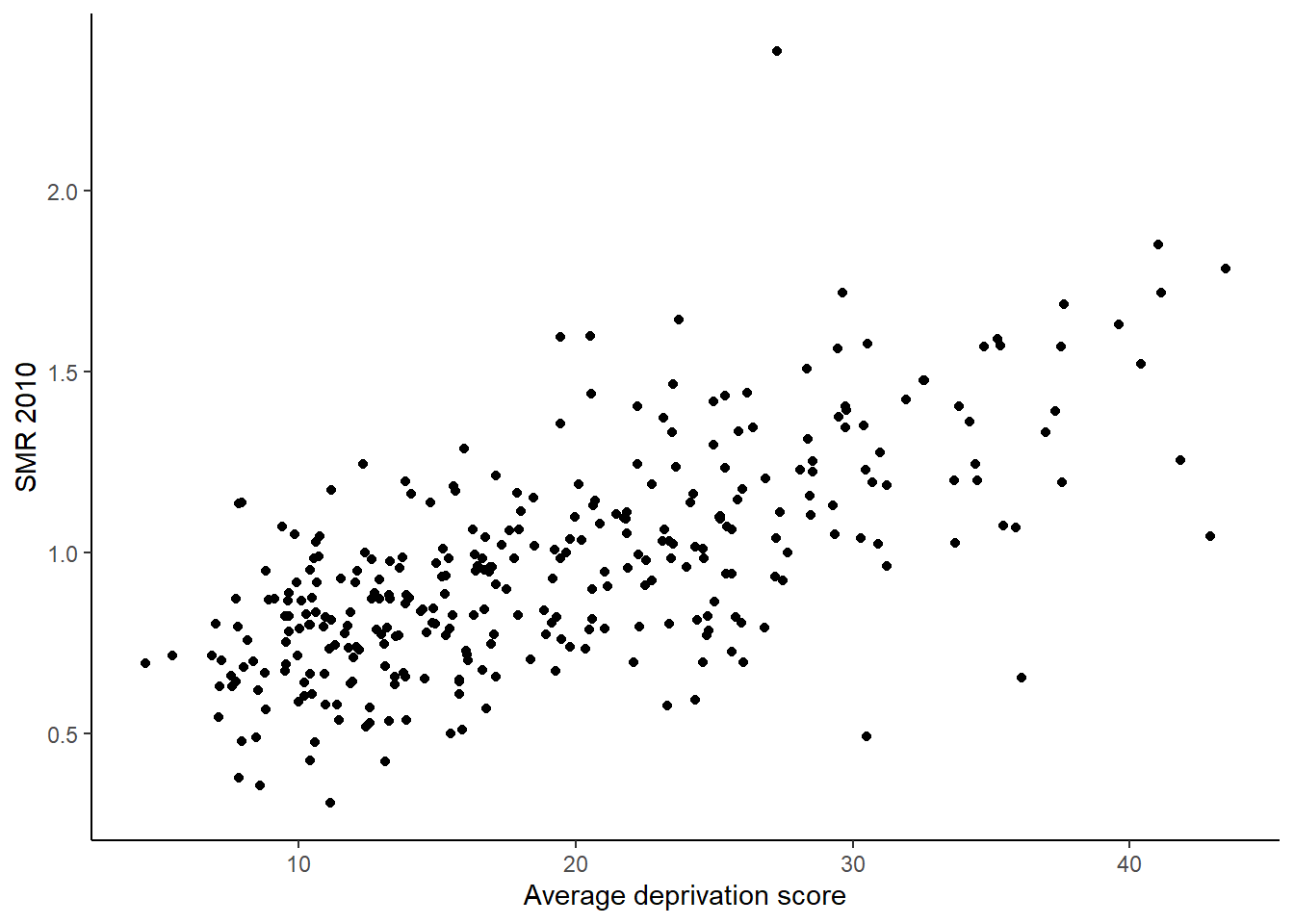
To fit the ICAR model in Nimble we need to obtain the neighborhood matrix \(W\). We start by defining a function that computes the number of neighbors for each
area.
adjlist = function(W, N) {
  adj = 0
  for (i in 1:N) {
    for (j in 1:N) {
      if (W[i, j] == 1) {
        adj = append(adj, j)
      }
    }
  }
  adj = adj[-1]
  return(adj)
}
Next we obtain the adjacency matrix, W,Define the adjacency matrix and indexes for stan using the functions nb2mat and adjlist from package spdep.
# Create the neighborhood
W.nb <-poly2nb(england, row.names = rownames(england))
# Creates a matrix for following function call
W.mat <- nb2mat(W.nb, style = "B")
# Define the spatial structure to use in stan
N <- length(unique(england$ID))
#creating a vector listing the ID numbers of the adjacent areas for each area
neigh  <- adjlist(W.mat, N)
# computing a vector of length N (the total number of areas) giving the number of neighbors for each area.
numneigh  <- apply(W.mat,2,sum)
Example9_3Nimble <- nimbleCode({
# Likelihood
for (i in 1:N) {
y[i] ~ dpois(lambda[i])
log(lambda[i]) <- log(E[i]) + b[i] + beta0 + beta1*x[i]
}
# Priors
beta0 ~ dnorm(0, sd = 1)
beta1 ~ dnorm(0, sd = 1)
b[1:N] ~ dcar_normal(adj[1:L], weights[1:L], num[1:N], tau, zero_mean = 1)
tau <- 1 / (sigma_b ^ 2)
#prior for sigma_b is a half-normal distribution
sigma_b ~ T(dnorm(0, sd = 1), 0,)
# Fitted values and likelihood for WAIC
for (i in 1:N) {
fitted[i] ~ dpois(lambda[i])
}
})
# Define the constants, data and initial values lists and run the model.
# constants list
constants <- list(
N = N,
E = copd_df$E2010,
L = length(neigh),
adj = neigh,
weights = rep(1, length(neigh)),
num = as.vector(numneigh),
p = 3
)
# data list
ex.data <-
list(y = copd_df$Y2010,
x = as.vector(copd_df$Average.Score)) # vector of covariates
inits <- list(
beta0 = rnorm(1),
beta1 = rnorm(1),
fitted = rpois(N, 2),
sigma_b = 1,
b = rnorm(N)
)
params <- c("beta0","beta1", "fitted", "b", "tau")
# Run model in nimble
mcmc.out <- nimbleMCMC(
code = Example9_3Nimble,
constants = constants,
data = ex.data,
inits = inits,
monitors = params,
niter = 40000,
nburnin = 20000,
thin = 20,
WAIC = TRUE,
nchains = 2,
summary = TRUE,
samplesAsCodaMCMC = TRUE
)Next we double-check convergence of the chains through trace plots and the effective sample sizes for some of the parameters.
## [1] 106.484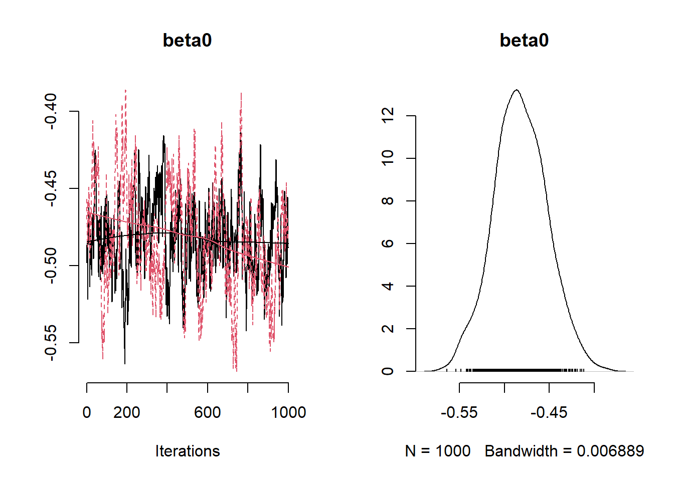
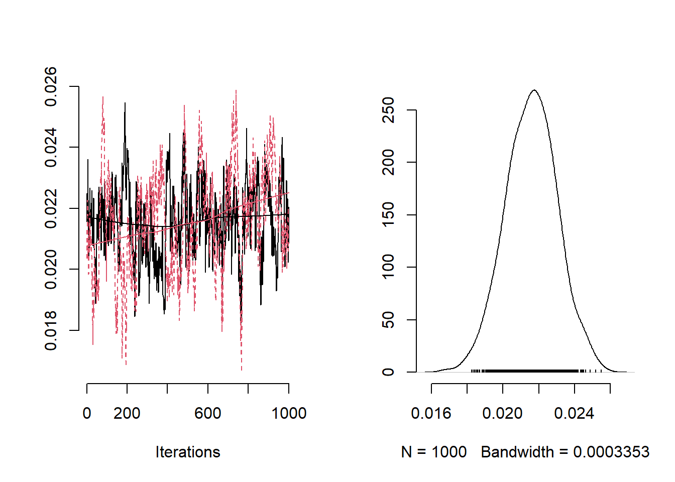
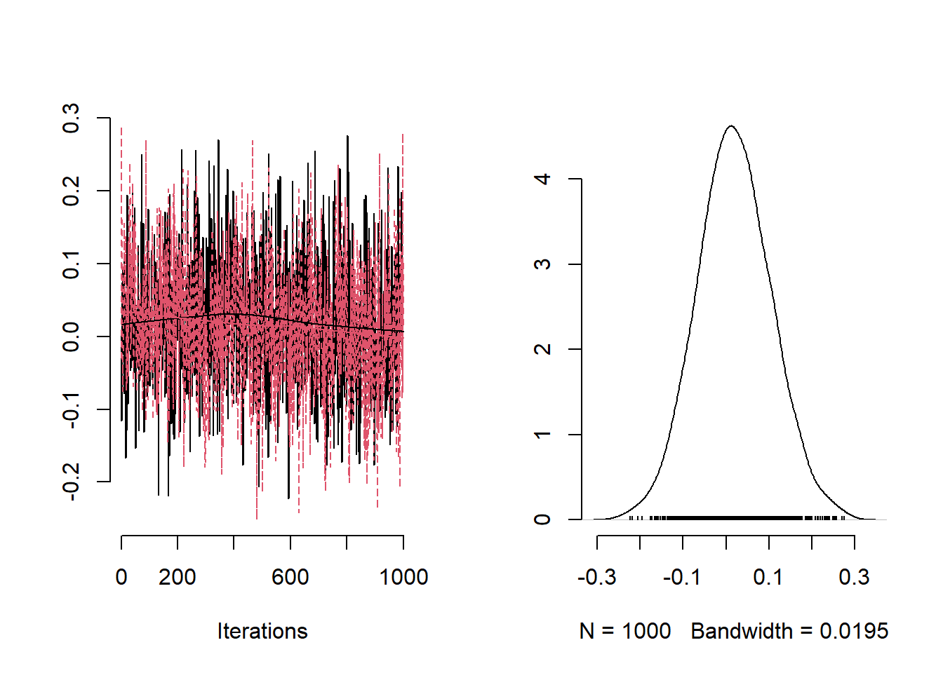
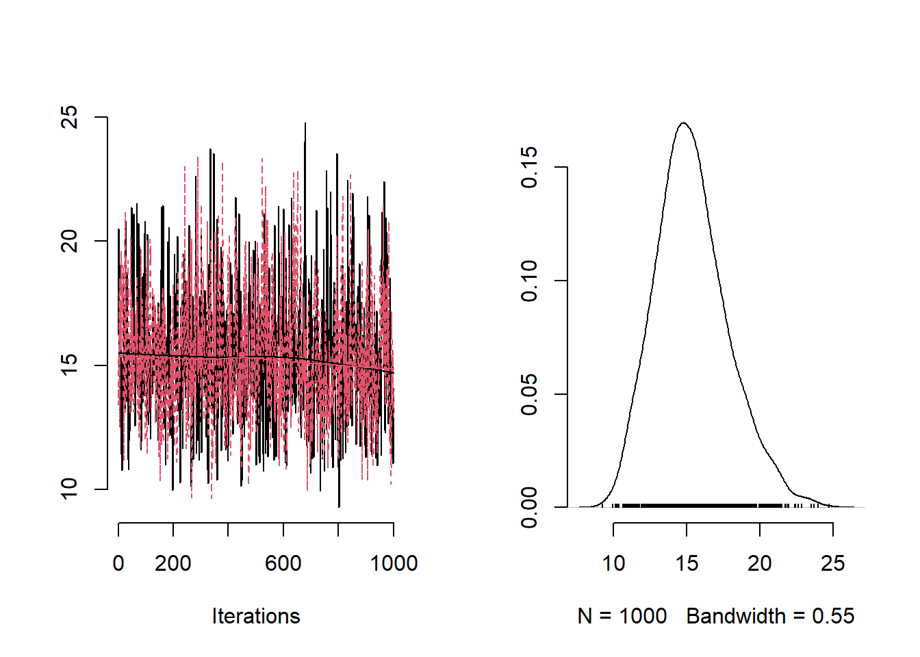
Posterior summaries of the intercept, the fixed effect for average deprivation index and the precision of the ICAR prior distribution.
# Extract samples
variables <- c("beta0", "beta1","tau")
summary_CAR_nimble <- mcmc.out$summary$all.chains
summary_CAR_nimble[variables,]
## Mean Median St.Dev. 95%CI_low 95%CI_upp
## beta0 -0.48208299 -0.48319524 0.029720605 -0.54251409 -0.42199775
## beta1 0.02158382 0.02160515 0.001446477 0.01868493 0.02446601
## tau 15.38297154 15.18218615 2.462509582 11.19231669 20.87252479Map of the posterior mean of the latent effects.
samples_CAR_b <-
  summary_CAR_nimble[grepl("b\\[", rownames(summary_CAR_nimble)), ] |> as.data.frame()
observed <- tibble::rownames_to_column(observed, "ID")
samples_CAR_b$ID <- observed$ID
CAR_nimble_merge <- merge(england, samples_CAR_b, by = "ID")
ggplot() +
  # Choose spatial object and column for plotting
  geom_sf(data = CAR_nimble_merge, aes(fill = Mean)) +
  # Change legend's label
  labs(fill = 'Latent effects under Nimble') +
  # Clear background and plot borders
 theme_void()
Now we perform the same analysis using Stan. Note that, different from Nimble, the sum-to-zero constraint in Stan is a soft one.
Stan
As Stan does not have a specific function for the ICAR prior we need to compute the neighborhood structure through the following functions which were obtained from this site:
adjlist = function(W, N) {
  adj = 0
  for (i in 1:N) {
    for (j in 1:N) {
      if (W[i, j] == 1) {
        adj = append(adj, j)
      }
    }
  }
  adj = adj[-1]
  return(adj)
}

mungeCARdata4stan = function(adjBUGS, numBUGS) {
  N = length(numBUGS)
  nn = numBUGS
  N_edges = length(adjBUGS) / 2
  node1 = vector(mode = "numeric", length = N_edges)
  node2 = vector(mode = "numeric", length = N_edges)
  iAdj = 0
  iEdge = 0

  for (i in 1:N) {
    for (j in 1:nn[i]) {
      iAdj = iAdj + 1
      if (i < adjBUGS[iAdj]) {
        iEdge = iEdge + 1
        node1[iEdge] = i
        node2[iEdge] = adjBUGS[iAdj]
      }
    }
  }
  return (list(
    "N" = N,
    "N_edges" = N_edges,
    "node1" = node1,
    "node2" = node2
  ))

}
This model is in a separate file called Example9_3.stan that will be called later.
data {
  int<lower=1> N;
  int<lower=1> N_edges;
  int<lower=1> p;
  matrix[N,p] X;
  int<lower=1, upper=N> node1[N_edges];  // node1[i] adjacent to node2[i]
  int<lower=1, upper=N> node2[N_edges];  // and node1[i] < node2[i]
  int<lower=0> y[N];              // count outcomes
  vector<lower=0>[N] E;           // exposure
}

transformed data {
  vector[N] log_E = log(E);

}

parameters {
  real beta0;            // intercept
  vector[p] beta;
  vector[N] s;         // spatial effects
  real<lower=0> sigma_s;        // marginal standard deviation of spatial effects
}

transformed parameters {
  vector[N] b; // latent effect
  real <lower=0> riskdep = exp(beta[1]);

  b =  sigma_s*s;
}

model {
  y ~ poisson_log(log_E + beta0 + X*beta + b);
  // This is the prior for s! (up to proportionality)
  target += -0.5 * dot_self(s[node1] - s[node2]);
  //soft sum-to-zero constraint
  sum(s) ~ normal(0, 0.001 * N);

  beta0 ~ normal(0.0, 10.0);
 for(j in 1:p){
    beta[j] ~ normal(0.0, 10.0);
  }
    sigma_s ~ normal(0.0,1.0);
}

generated quantities {
  vector[N] mu=exp(log_E + beta0  + X*beta + b);
  vector[N] lik;
  vector[N] log_lik;

  for(i in 1:N){
    lik[i] = exp(poisson_lpmf(y[i] | mu[i] ));
    log_lik[i] = poisson_lpmf(y[i] | mu[i] );
  }
}
Define the adjacency matrix and the set of indices of the neighboring areas using functions nb2mat and adjlist:
# Create the neighborhood
W.nb <-
  poly2nb(england, row.names = rownames(england))
# Creates a matrix for following function call
W.mat <- nb2mat(W.nb, style = "B")

# Define the spatial structure to use in stan
N <- length(unique(england$ID))
neigh <- adjlist(W.mat, N)
numneigh  <-  apply(W.mat, 2, sum)
nbs <- mungeCARdata4stan(neigh, numneigh)


# Define data and variables for Stan model
y <- copd_df$Y2010
E <- copd_df$E2010
X <- as.numeric(copd_df$Average.Score)

ex.data <- list(
  N =  nbs$N,
  y = y,
  E = E,
  p = 1,
  X = as.matrix(X),
  N_edges = nbs$N_edges,
  node1 = nbs$node1,
  node2 = nbs$node2
)

Example9_3Stan  <- stan(
  file = "functions/Example9_3.stan",
  data = ex.data,
  warmup = 2000,
  iter = 10000,
  chains = 2,
  thin = 8,
  pars = c("beta0", "beta","sigma_s", "riskdep", "b", "log_lik"),
  include = TRUE
)
Trace plots of the posterior samples for some of the parameters.
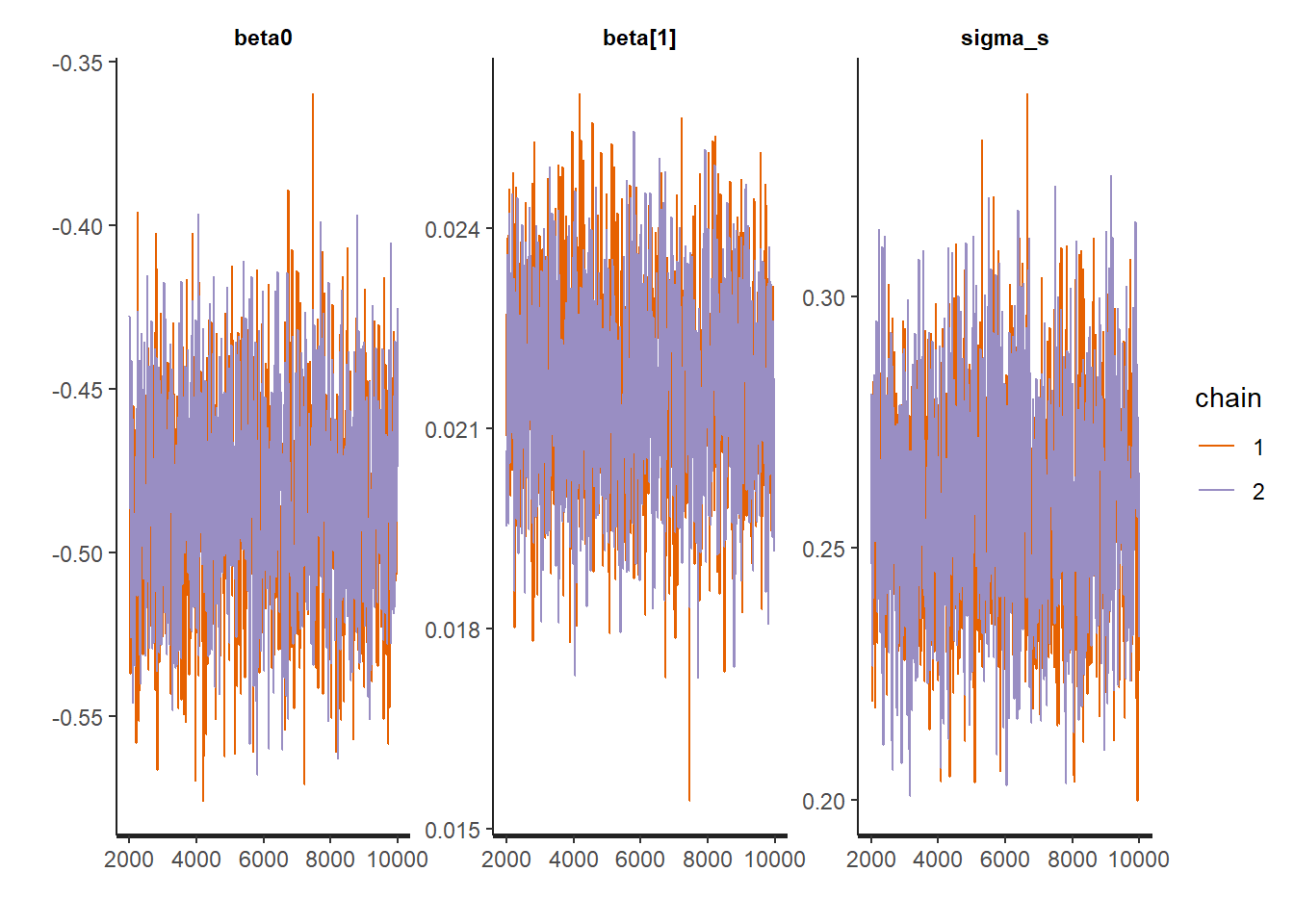
We now obtain the posterior summaries of the intercept, the fixed effect associated with the deprivation score and the standard deviation of the random effect. The quantity riskdep shows the relative risk associated with an one unit increase in deprivation.
# Extract samples
summary_CAR_stan <-
  summary(
    Example9_3Stan,
    pars = c("beta0", "beta","sigma_s","riskdep"),
    probs = c(0.025, 0.975)
  )

summary_CAR_stan$summary
## mean se_mean sd 2.5% 97.5% n_eff
## beta0 -0.4831513 7.614790e-04 0.029746646 -0.54094962 -0.42631806 1526.020
## beta[1] 0.0216228 3.757970e-05 0.001446513 0.01884916 0.02450198 1481.623
## sigma_s 0.2581699 5.230906e-04 0.021200471 0.21816947 0.30228148 1642.621
## riskdep 1.0218593 3.840191e-05 0.001478135 1.01902793 1.02480462 1481.572
## Rhat
## beta0 1.000210
## beta[1] 1.000255
## sigma_s 1.000640
## riskdep 1.000257The result suggests that an one unit increase in deprivation, increases the relative risk by 2.2%. Recall that the standard deviation of the ICAR prior refers to the standard deviation of a conditional distribution.
We now plot the posterior means of the latent effects
summary_CAR_stan_b <-
  summary(
    Example9_3Stan,
    pars = c("b"),
    probs = c(0.025, 0.975)
  )

observed <- tibble::rownames_to_column(observed, "ID")

summary_CAR_stan_b$ID <- observed$ID

CAR_stan_merge <- merge(england, summary_CAR_stan_b, by = "ID")

ggplot() +
  # Choose spatial object and column for plotting
  geom_sf(data = CAR_stan_merge, aes(fill = summary.mean)) +
  # Change legend's label
  labs(fill = 'Latent effects stan') +
  # Clear background and plot borders
  theme_void()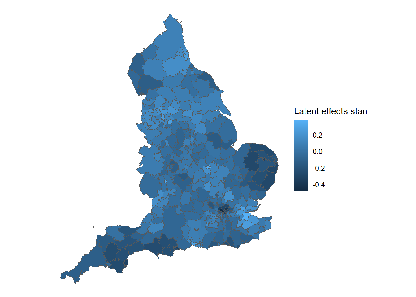
Example 9.4: Fitting a conditional spatial model using CARBayes
Here we consider fitting the Poisson log–normal model with spatial effects to the data for respiratory admissions seen in Example 9.3 using the R package CARBayes. The adjacency matrix is obtained using functions of the package spdep.
CARBayes performs MCMC simulation similar to NIMBLE but has the distinct advantage that you just call specific functions to run the model.
library(CARBayes)
library(ggplot2)
library(sf)
library(spdep)

# Reading in borders
england <- read_sf("data/copd/englandlocalauthority.shp")
# Reading in data
observed <-
  read.csv(file = "data/copd/copdmortalityobserved.csv", row.names = 1)
expected <-
  read.csv(file = "data/copd/copdmortalityexpected.csv")
covariates <- read.csv(file = "data/copd/copdavgscore.csv")
# Merge everything into one data frame
copd_df <-
  cbind(observed,  expected) |> merge(
    covariates,
    by.x = "code",
    by.y = "LA.CODE",
    all.x = TRUE,
    all.y = FALSE
  )
copd_df$Average.Score <- as.numeric(scale(copd_df$Average.Score))
Next we compute the neighborhood matrix through poly2nb() and nb2mat() from the spdep.
# Create the neighborhood
W.nb <-poly2nb(england, row.names = rownames(england))

# Creates a matrix for following function call
W.mat <-  nb2mat(W.nb, style = "B")
The function S.CARleroux() allows us to use the neighborhood structure and performs a Bayesian analysis assuming a CAR prior distribution to the random effects. This is obtained by setting the parameter rho equals 1 in the call of S.CARleroux().
# Running smoothing model
Ex9_4 <-
  S.CARleroux(
    # Model Formula
    formula = Y2010 ~ offset(log(E2010)) + Average.Score,
    # data frame with data
    data = copd_df,
    # Choosing Poisson Regression
    family = "poisson",
    # Neighborhood matrix
    W = W.mat,
    # Number of burn in samples
    burnin = 20000,
    # Number of MCMC samples
    n.sample = 100000,
    thin = 10,
    #ICAR model given a 0-1 neighborhood structure
    rho = 1
  )
Using ggplot() and geom_sf() to plot the map of the latent spatial effects.
observed <- tibble::rownames_to_column(observed, "ID")
phi_car <-  Ex9_4$samples$phi

latent_car_df  <-  data.frame(
  phi_mean = apply(phi_car, 2, mean),
  phi_sd = apply(phi_car, 2, sd)
)
# Combine latent spatial effect with england dataset
latent_car_df$ID <- observed$ID
latent_car_england <-  merge(england, latent_car_df, by = "ID")
# Creating map of smoothed SMRs in England in 2010
ggplot() +
  # Choose spatial object and column for plotting
  geom_sf(data = latent_car_england, aes(fill = phi_mean)) +
  labs(fill = 'Latent effects CARbayes') +
  # Clear background and plot borders
  theme_void()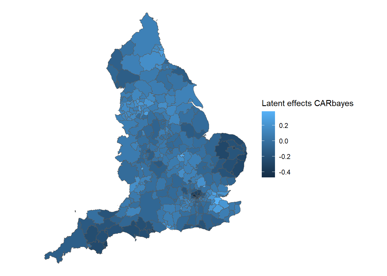
Example 9.5: Fitting a conditional model using INLA
Now we fit the Poisson log–normal model with spatial effects to the data for respiratory admissions seen in Example 9.3 using R-INLA. Recall that R-INLA approximates the resultant posterior distribution using an integrated nested Laplace approximation. The call to fit the model using R-INLA is very similar to the one when fitting a glm. The latent effects are introduced through the function f(.).
# run the INLA model
Ex9_5 <- inla(
  Y2010 ~ Average.Score + f(ID  , model = "besag", graph = "UK.adj"),
  family = "poisson",
  E = E2010,
  data = copd_df,
  control.predictor = list(compute = TRUE)
)
Summarize the results
##
## Call:
##    c("inla.core(formula = formula, family = family, contrasts = contrasts,
##    ", " data = data, quantiles = quantiles, E = E, offset = offset, ", "
##    scale = scale, weights = weights, Ntrials = Ntrials, strata = strata,
##    ", " lp.scale = lp.scale, link.covariates = link.covariates, verbose =
##    verbose, ", " lincomb = lincomb, selection = selection, control.compute
##    = control.compute, ", " control.predictor = control.predictor,
##    control.family = control.family, ", " control.inla = control.inla,
##    control.fixed = control.fixed, ", " control.mode = control.mode,
##    control.expert = control.expert, ", " control.hazard = control.hazard,
##    control.lincomb = control.lincomb, ", " control.update =
##    control.update, control.lp.scale = control.lp.scale, ", "
##    control.pardiso = control.pardiso, only.hyperparam = only.hyperparam,
##    ", " inla.call = inla.call, inla.arg = inla.arg, num.threads =
##    num.threads, ", " blas.num.threads = blas.num.threads, keep = keep,
##    working.directory = working.directory, ", " silent = silent, inla.mode
##    = inla.mode, safe = FALSE, debug = debug, ", " .parent.frame =
##    .parent.frame)")
## Time used:
##     Pre = 1.02, Running = 0.289, Post = 0.108, Total = 1.42
## Fixed effects:
##                 mean    sd 0.025quant 0.5quant 0.975quant   mode kld
## (Intercept)   -0.069 0.008     -0.084   -0.069     -0.054 -0.069   0
## Average.Score  0.182 0.012      0.158    0.182      0.206  0.182   0
##
## Random effects:
##   Name     Model
##     ID Besags ICAR model
##
## Model hyperparameters:
##                   mean   sd 0.025quant 0.5quant 0.975quant  mode
## Precision for ID 15.94 2.62      11.52    15.70      21.75 15.23
##
## Marginal log-Likelihood:  -1493.27
##  is computed
## Posterior summaries for the linear predictor and the fitted values are computed
## (Posterior marginals needs also 'control.compute=list(return.marginals.predictor=TRUE)')
observed <- tibble::rownames_to_column(observed, "ID")
phi_car <- Ex9_5$summary.random$ID
latent_car_df <- data.frame(
phi_mean = phi_car$mean,
phi_sd = phi_car$sd
)
# Combine latent spatial effect with england dataset
latent_car_df$ID <- observed$ID
latent_car_england <- merge(england, latent_car_df, by = "ID")
# Creating map of smoothed SMRs in England in 2010
ggplot() +
# Choose spatial object and column for plotting
geom_sf(data = latent_car_england, aes(fill = phi_mean)) +
labs(fill = 'Latent effects INLA') +
# Clear background and plot borders
theme_void()