Chapter 7 Strategies for modelling
This chapter considers both some wider issues related to modelling and the generalisability of results, together with more technical material on the effect of covariates and model selection. The reader will have gained an understanding of the following topics:
why having contrasts in the variables of interest is important in assessing the effects they have on the response variable;
biases that may arise in the presence of covariates and how covariates can affect variable selection and model choice;
hierarchical models and how that can be used to acknowledge dependence between observations;
the issues associated with the use of p-values as measures of evidence against a null hypothesis and why basing scientific conclusions on it can lead to non-reproducible results;
use of predictions from exposure models, including acknowledging the additional uncertainty involved when using predictions as inputs to a health model;
methods for performing model selection, including the pros and cons of automatic selection procedures;
model selection within the Bayesian setting, and how the models themselves can be incorporated into the estimation process using Bayesian Model Averaging.
Example 7.6 Variable selection in land use regression using lasso and horseshoe priors
This example is based on the Volatile Organic Compound (VOC) data analyzed by Zapata-Marin et al. (2022). VOCs are components of the complex mixture of air pollutants within cities and can cause various adverse health effects. VOCs concentrations were measured over 2-week periods, for three monitoring campaigns between 2005 and 2006 across over 130 locations in Montreal, QC, Canada. The data analyzed in this example is ethylbenzene observed during April 2006.
Land-use variables were available as a proportion of the area of each buffer covered by each specific variable. In this example, we explore the land-use variables using circular buffers at 1,000-m radii around each monitoring location. The land use variables include Building_100m,Government and Institutional, Residential, Population,Roads,Total NOx.
Below we read the data and plot the monitoring locations with solid circles proportional to the observed value of ethylbenzene.
library(dplyr)
library(geoR)
library(GGally)
library(leaflet)
library(ggplot2)
library(sp)
library(spdep)
library(nimble)
# Load data on benzene concentration in Montreal
ethylbenzene <- read.csv("data/montreal_ethylbenzene.csv")
We start by mapping the locations of the monitoring sites across Montreal. The diameter of the circles are proportional to the observed concentration of ethylbenzene.
range_values <- range(log(ethylbenzene$Ethylbenzene))

# Define bins based on the range of values
mybins <- seq(range_values[1], range_values[2], length.out = 5)

mypalette <- colorBin(palette="inferno", domain=ethylbenzene$Ethylbenzene,
                      na.color="transparent", bins=mybins)

leaflet( data = ethylbenzene) |>
  addTiles()  |>
  addProviderTiles("Esri.WorldImagery")  |>
  addCircleMarkers(
    ~ lon,
    ~ lat,
    fillOpacity = 0.8, color="orange",
    fillColor = ~ mypalette(log(Ethylbenzene)),
    opacity = 5,
    radius = ~log(Ethylbenzene)*4,
    stroke = FALSE) |>
  addLegend( pal=mypalette, values=~log(Ethylbenzene),
             opacity=0.9, title = "log(Ethylbenzene)", position = "bottomright" )
We now perform a simple exploratory data analysis using the ggpairs command. It provides the empirical distribution of each of the variables as well as pairwise correlations among them. We transform two variables, Building and Total NOx to obtain a more symmetric empirical distributions. The greatest observed correlation among the variables is 0.614, between Roads and Population.
##  [1] "X"                                  "Y"
##  [3] "ID"                                 "Building_100m"
##  [5] "Government.and.Institutional_1000m" "Residential_1000m"
##  [7] "Pop_1000m"                          "Roads_1000m"
## [9] "Tot_NOx_1000m" "Ethylbenzene"lur$X <- lur$X/1000
lur$Y <- lur$Y/1000
lur$lbuild<-sqrt(lur$Building_100m)
lur$lNOx<-log(lur$Tot_NOx_1000m)#removing X, Y, ID, Building_100m and Tot_NOx_1000m from the plot
ggpairs(lur[,-c(1:3,4,9)], title="correlogram with ggpairs()", progress = FALSE)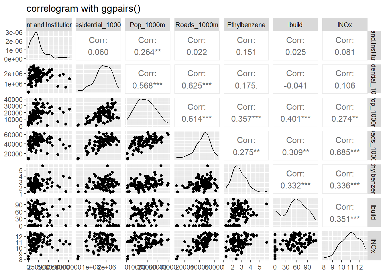
We now fit a linear model to the log(Ethylbenzene) that includes the log of buildings, government and institutional buildings, residential areas, population, roads and log of NOx:
#lur_ethyl <- lur |> select( ends_with("0m"), "X", "Y","Ethylbenzene")

# Fit a glm

fit_glm<-glm(log(Ethylbenzene) ~ X + Y  +
    lbuild +  Government.and.Institutional_1000m + Residential_1000m +
    Pop_1000m + Roads_1000m+lNOx, data = lur )
summary(fit_glm)
##
## Call:
## glm(formula = log(Ethylbenzene) ~ X + Y + lbuild + Government.and.Institutional_1000m +
## Residential_1000m + Pop_1000m + Roads_1000m + lNOx, data = lur)
##
## Deviance Residuals:
## Min 1Q Median 3Q Max
## -0.70723 -0.18976 0.00957 0.17620 0.59346
##
## Coefficients:
## Estimate Std. Error t value Pr(>|t|)
## (Intercept) 4.416e+00 2.229e+01 0.198 0.8434
## X -6.006e-03 5.088e-03 -1.180 0.2409
## Y -2.087e-04 4.729e-03 -0.044 0.9649
## lbuild 2.542e-03 9.912e-04 2.565 0.0120 *
## Government.and.Institutional_1000m 5.939e-09 1.410e-07 0.042 0.9665
## Residential_1000m 1.061e-07 8.989e-08 1.180 0.2410
## Pop_1000m 9.442e-06 4.908e-06 1.924 0.0575 .
## Roads_1000m -8.235e-06 5.967e-06 -1.380 0.1710
## lNOx 9.982e-02 4.689e-02 2.129 0.0359 *
## ---
## Signif. codes: 0 '***' 0.001 '**' 0.01 '*' 0.05 '.' 0.1 ' ' 1
##
## (Dispersion parameter for gaussian family taken to be 0.06620174)
##
## Null deviance: 8.4070 on 99 degrees of freedom
## Residual deviance: 6.0244 on 91 degrees of freedom
## AIC: 22.852
##
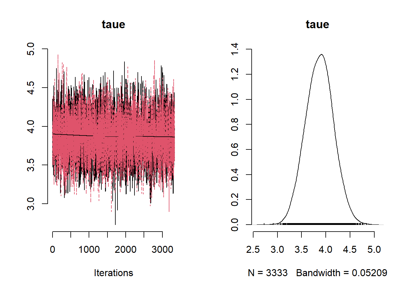
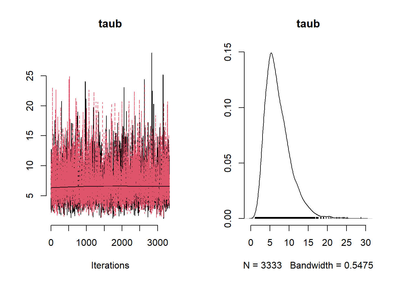
## Number of Fisher Scoring iterations: 2Variables log(building), population and lNOx are positively associated with log(Ethylbenzene). We now fit a linear model in Nimble using a Lasso prior for the coefficients of the variables.
Nimble
Ex7_6LassoCode <- nimbleCode({
  # Likelihood
  for (i in 1:n) {
    y[i]   ~ dnorm(mu[i], sd = sigma)
    mu[i] <- beta0 + inprod(X[i, ], beta[1:p])
  }

  # Prior specification
  for (j in 1:p) {
    beta[j] ~ ddexp(0, scale = 1/(taub * taue))
  }

  taue  ~  dgamma(0.1, 0.1)
  sigma <- 1/taue
  taub  ~  dgamma(0.1, 0.1)
  beta0  ~ dnorm(0, 10)

})
X <- lur |> dplyr::select( "lbuild", "Government.and.Institutional_1000m","Residential_1000m",
"Pop_1000m","Roads_1000m","lNOx", "X", "Y")
constants <-
list(n = nrow(lur), p = ncol(X))
ex.data <-
list(y = log(lur$Ethylbenzene),
X = scale(X))
params <- c( "beta0", "beta", "taub","taue", "sigma")
inits <- list( sigma = 0.1, tau = 0.1)
# Run model in nimble
start_time <- Sys.time()
mcmc.out.lasso <- nimbleMCMC(
code = Ex7_6LassoCode,
constants = constants,
data = ex.data,
inits = inits,
monitors = params,
niter = 100000,
nburnin = 50000,
thin = 15,
WAIC = TRUE,
nchains = 2,
summary = TRUE,
samplesAsCodaMCMC = TRUE
)
end_time <- Sys.time()
run_time <- end_time - start_time
run_time## [1] 4028.613
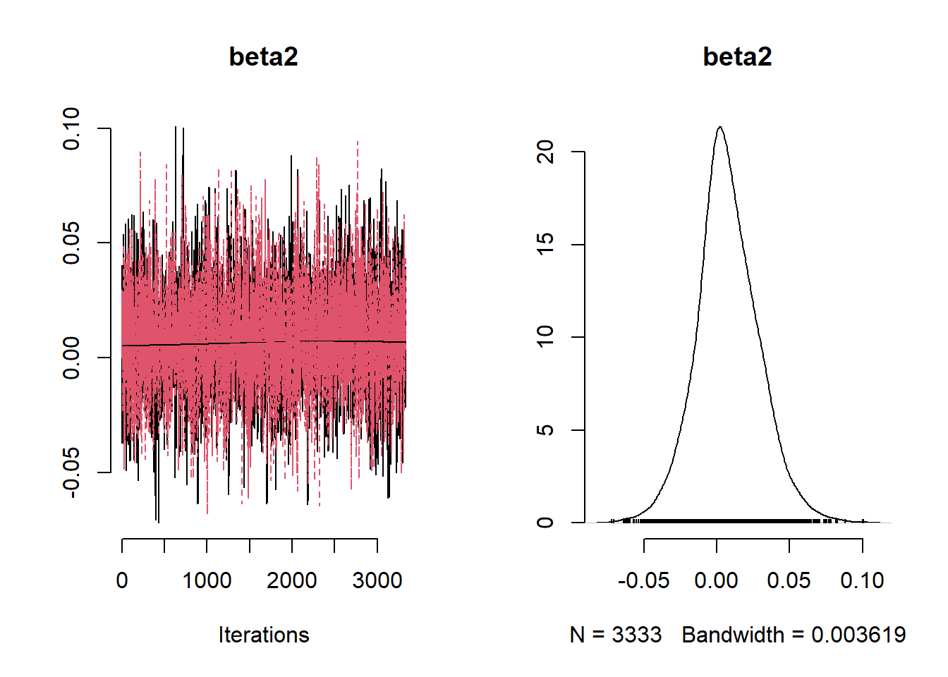
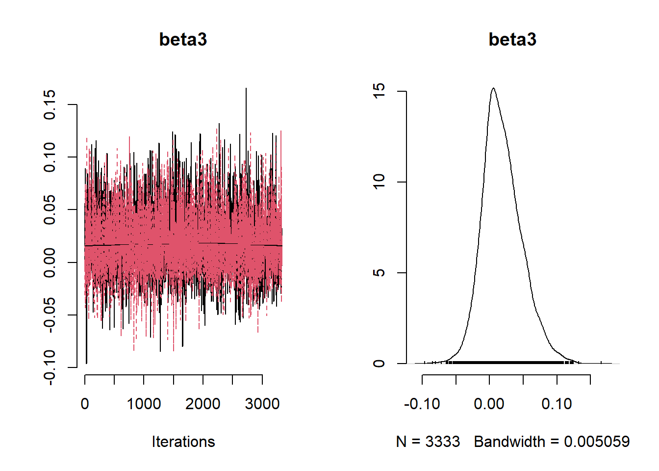
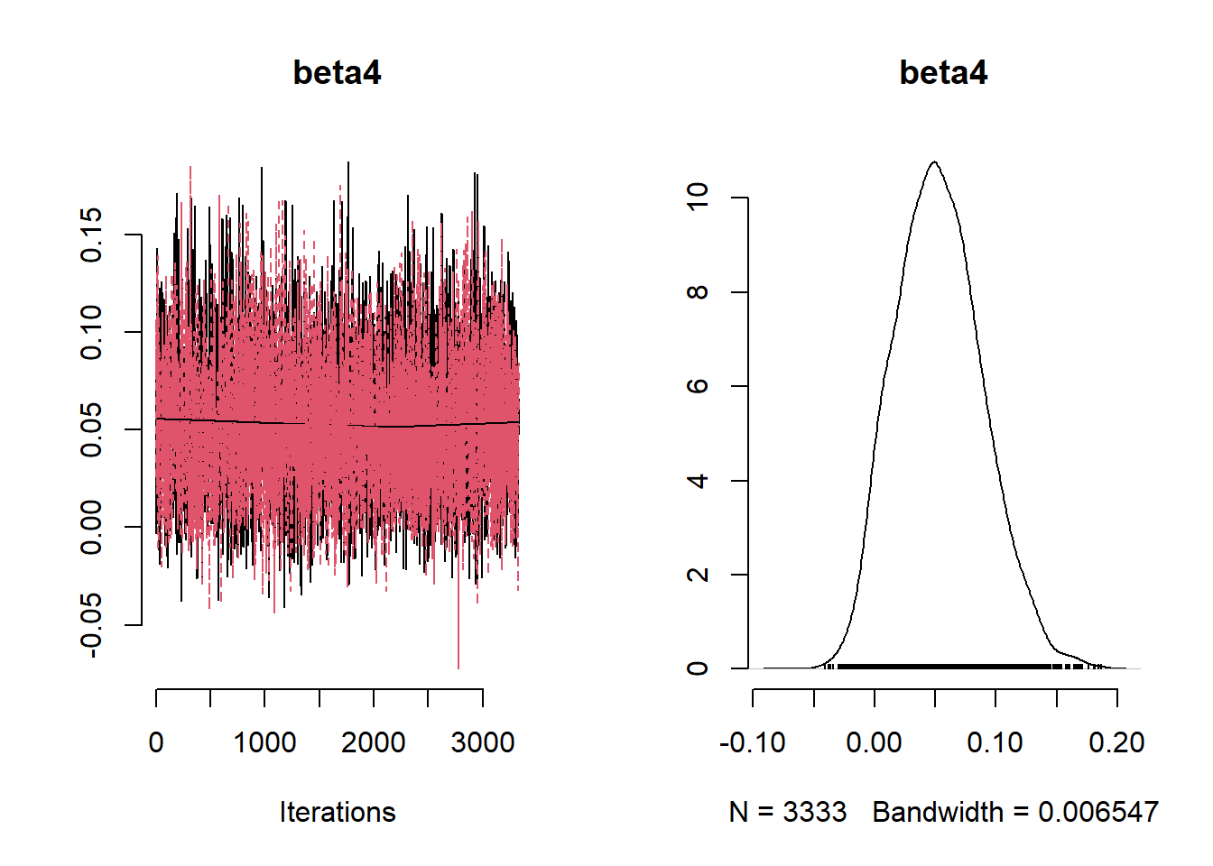
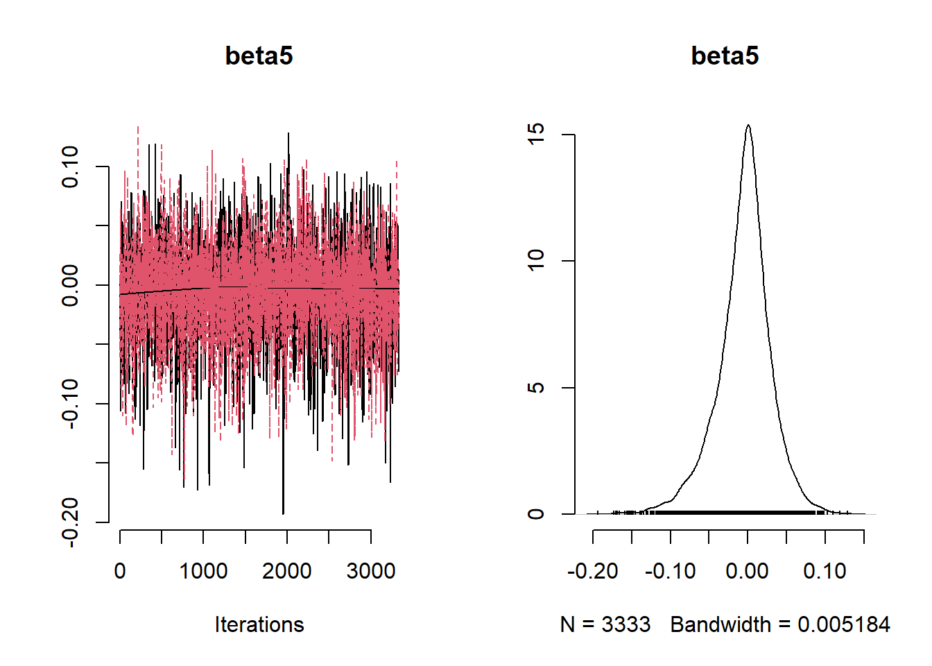
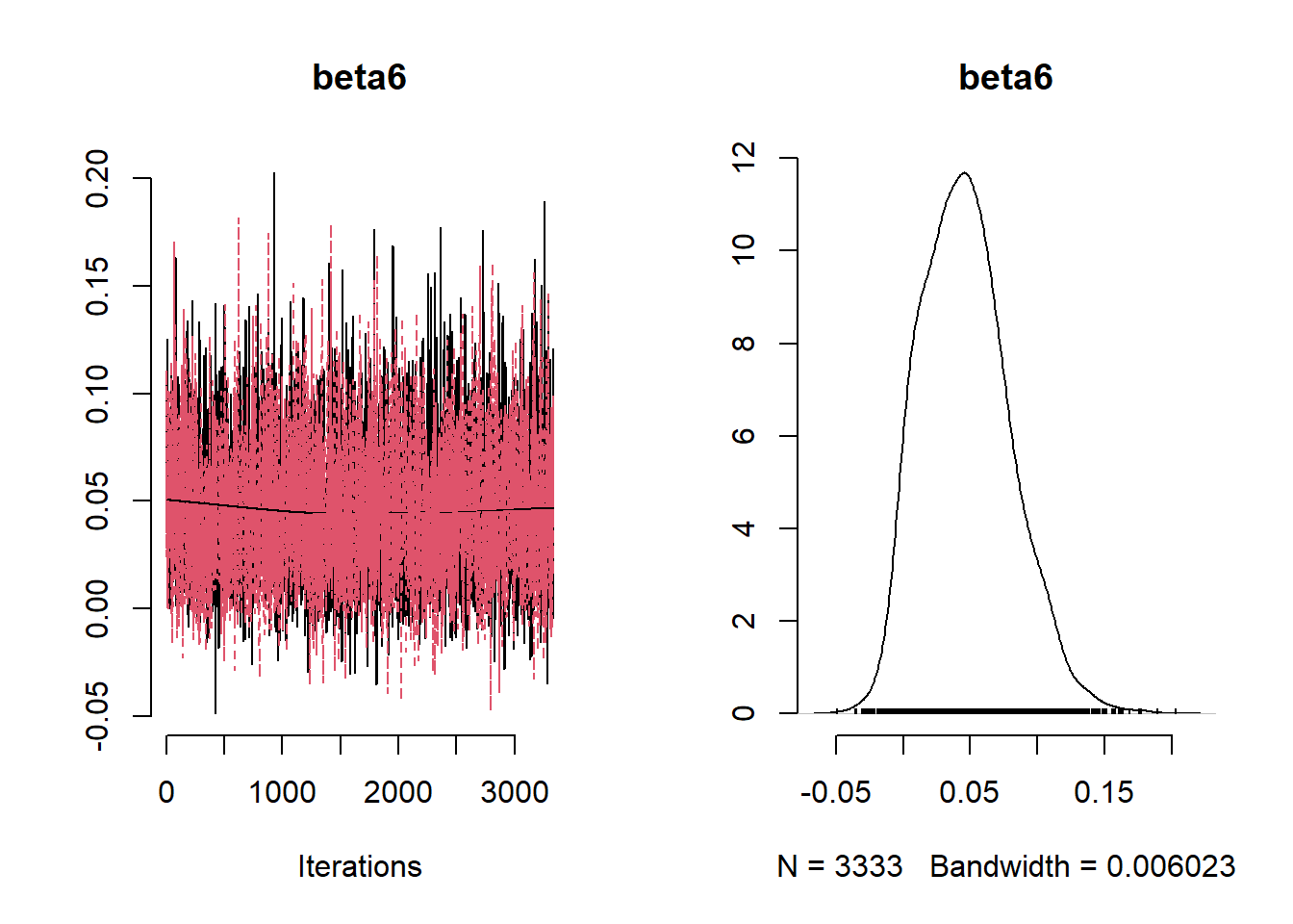
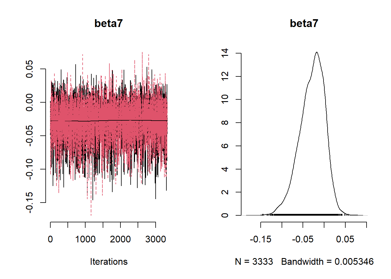
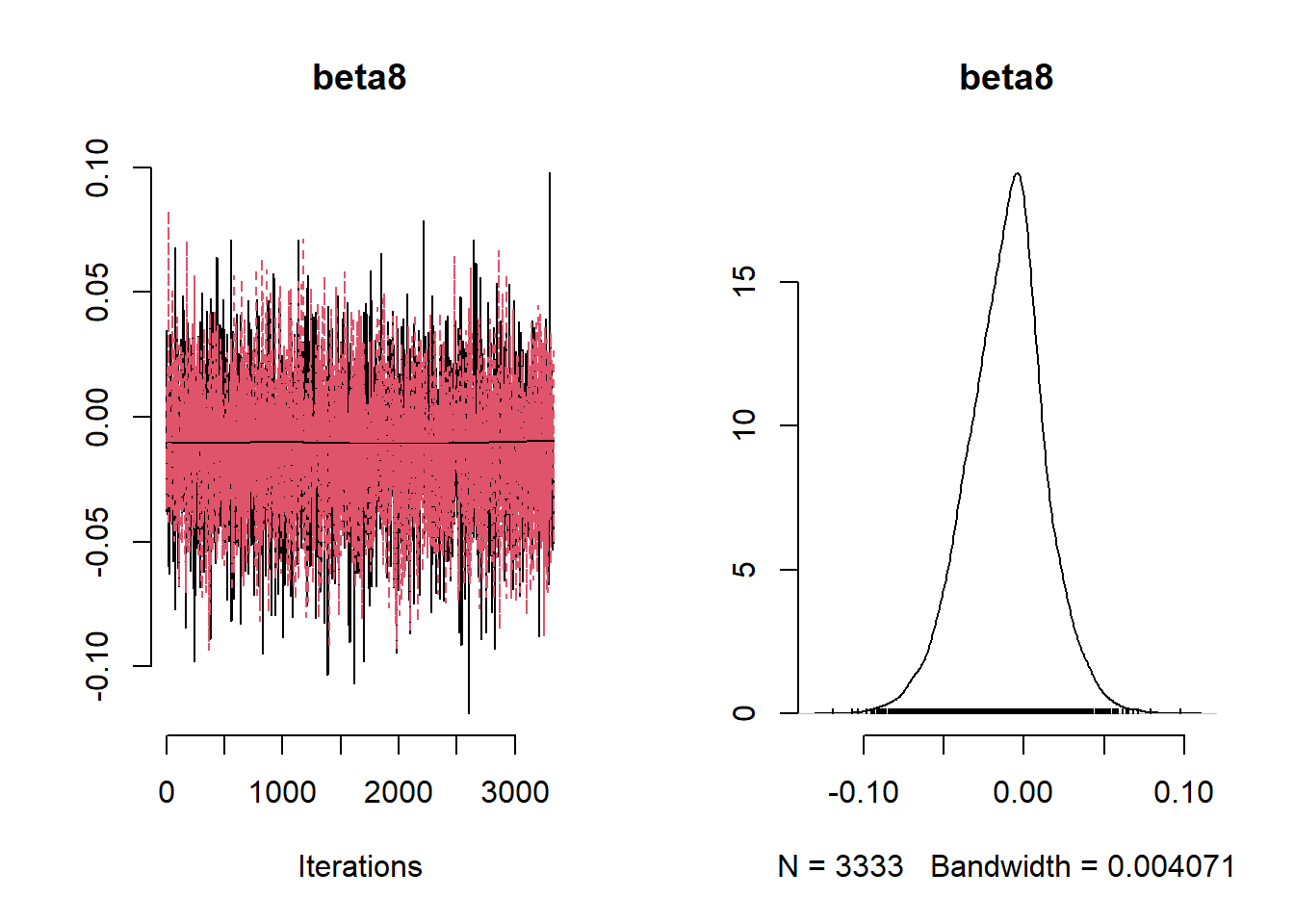
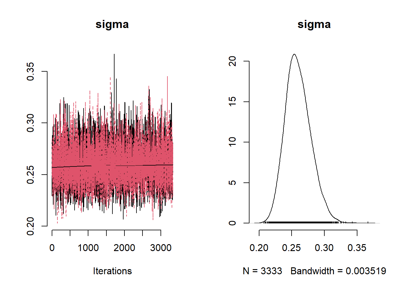
beta_var  <- paste0("beta[", 1:ncol(X), "]")
#posterior summaries of all the parameters in the model
post_summary_lasso <- mcmc.out.lasso$summary$all.chains |> as.data.frame()
post_summary_lasso <- post_summary_lasso[beta_var,]

post_summary_lasso$variable <- colnames(X)

ggplot(post_summary_lasso,
       aes(x = variable)) +
  geom_pointrange(aes(y = Mean, ymin =`95%CI_low`, ymax =`95%CI_upp`)) +
  geom_hline(yintercept = 0) +
  theme_classic() + theme(axis.text.x = element_text(angle = 90, vjust = 0.5, hjust=1))
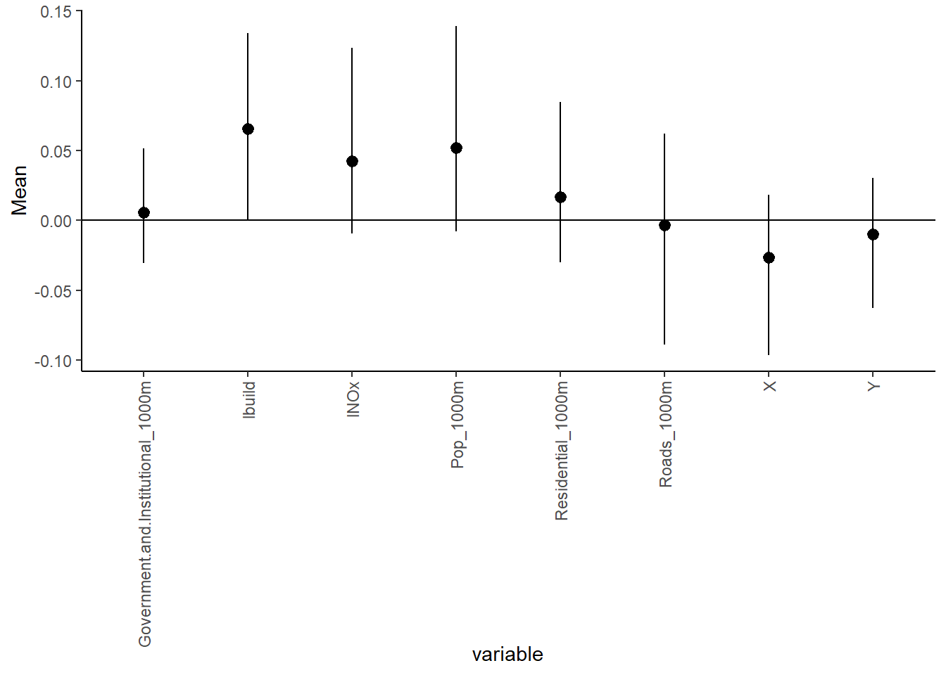
Under the Lasso prior specification, only the logarithm of Building_100m is associated with the logarithm of ethylbenzene.
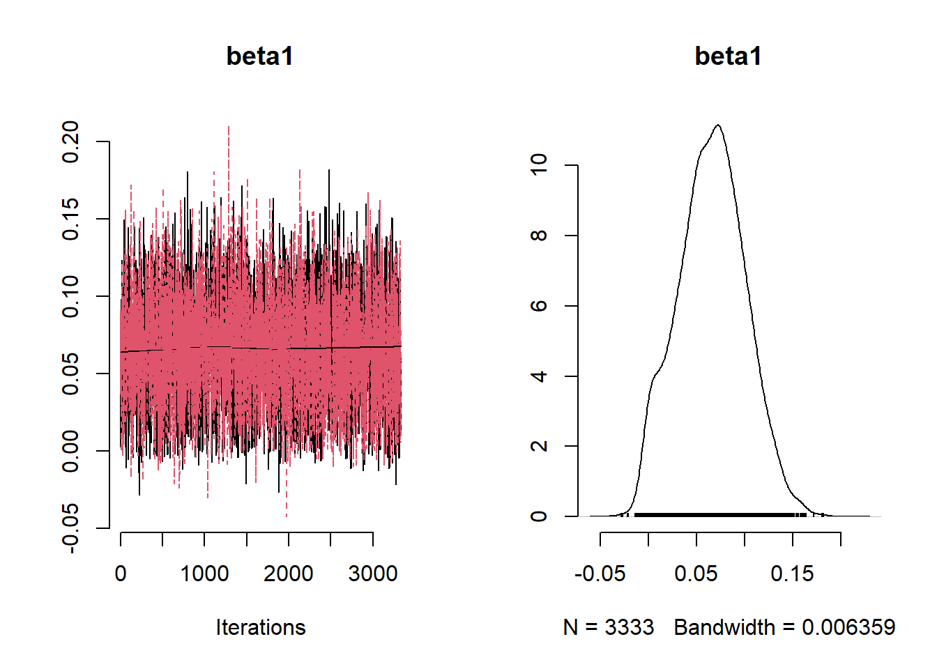
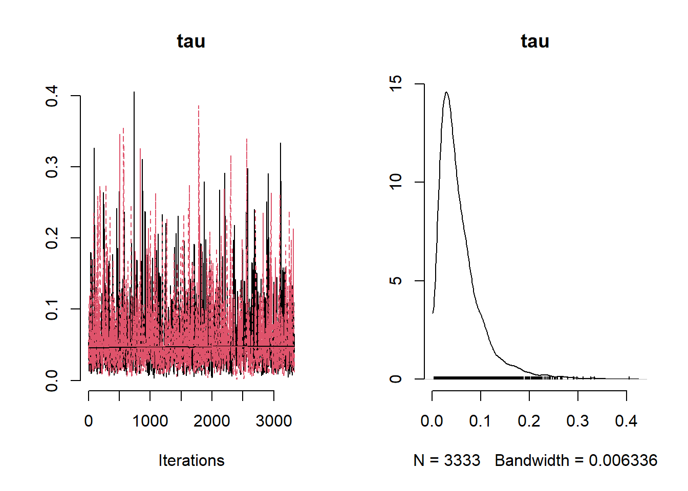
Next, we perform the analysis assuming a horseshoe prior for the coefficient.:
Ex7_6HorseshoeCode <- nimbleCode({

  # Likelihood
  for(i in 1:n){
    y[i]   ~ dnorm(mu[i], sd = sigma)
    mu[i] <- beta0 + inprod(X[i,], beta[1:p])
  }

  # Prior specification
  for(j in 1:p){
    beta[j] ~ dnorm(0, sd = lambda[j]*tau)
    lambda[j] ~ T(dt(mu = 0, sigma = 1, df = 1), 0, Inf)
  }
  tau  ~ T(dt(mu = 0, sigma = 1, df = 1), 0, Inf)
  sigma  ~ T(dt(mu = 0, sigma = 1, df = 1), 0, Inf)
  beta0  ~ dnorm(0,sd=10)

})set.seed(321)
constants <-
list(n = nrow(lur), p = ncol(X))
#using the scaled covariates
ex.data <-
list(y = log(lur$Ethylbenzene),
X = scale(X))
params <- c( "beta0", "beta", "tau", "sigma", "lambda")
inits <- list( sigma = 0.1, tau = 0.1)
# Run model in nimble
start_time <- Sys.time()
mcmc.out.hs <- nimbleMCMC(
code = Ex7_6HorseshoeCode,
constants = constants,
data = ex.data,
inits = inits,
monitors = params,
niter = 100000,
nburnin = 50000,
thin = 15,
WAIC = TRUE,
nchains = 2,
summary = TRUE,
samplesAsCodaMCMC = TRUE
)
end_time <- Sys.time()
run_time <- end_time - start_time
run_time## [1] 661.5456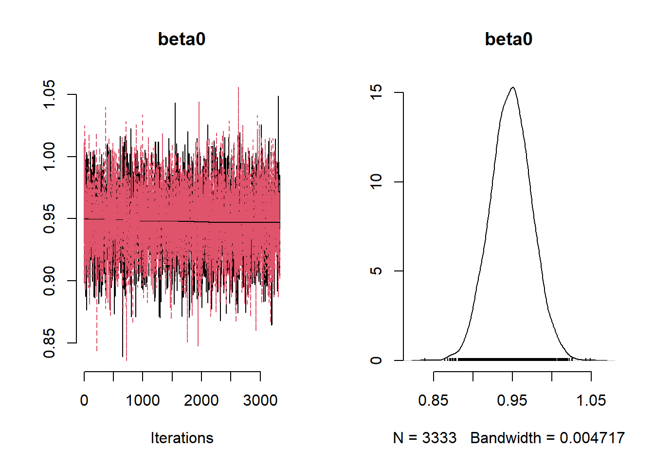
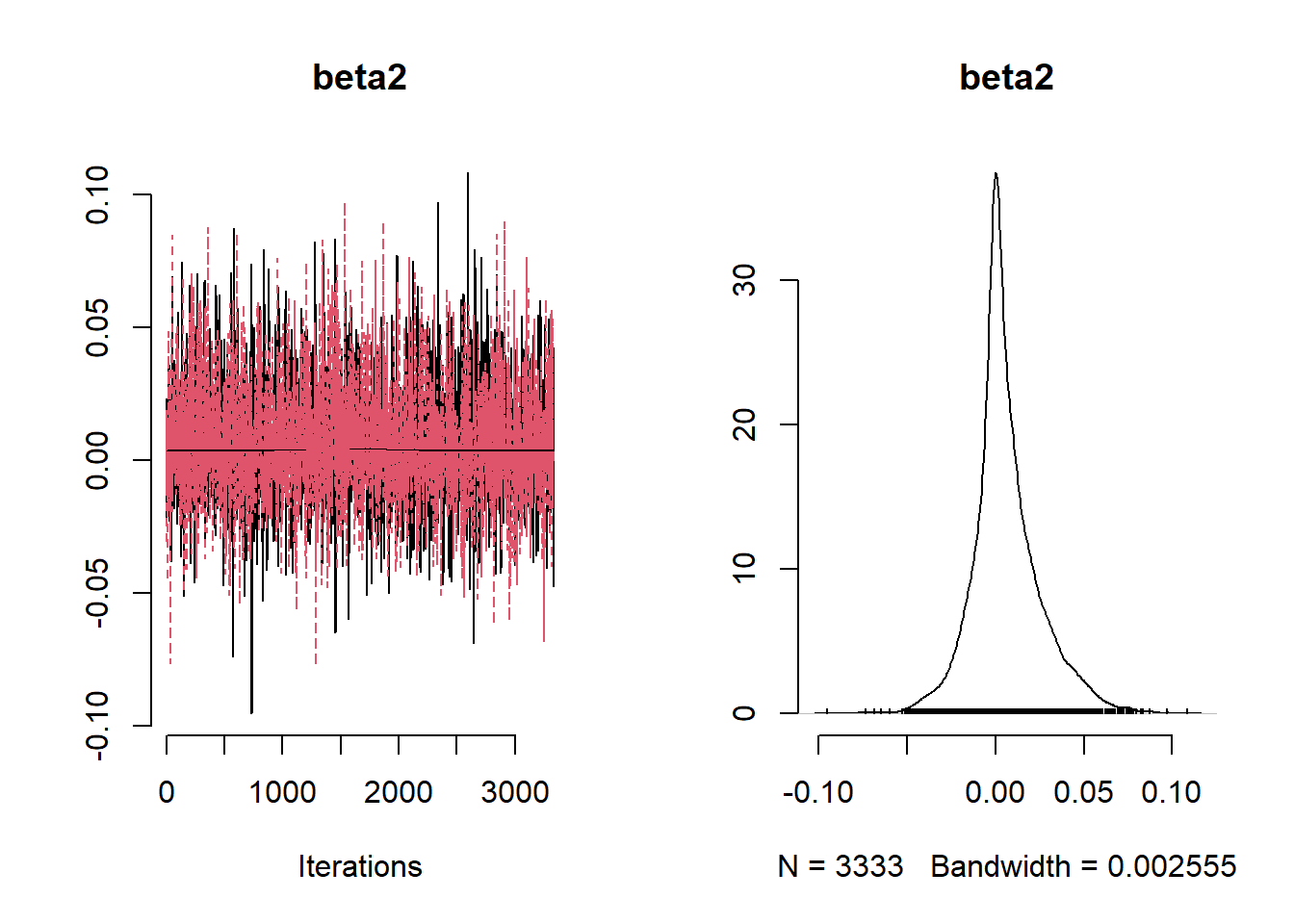
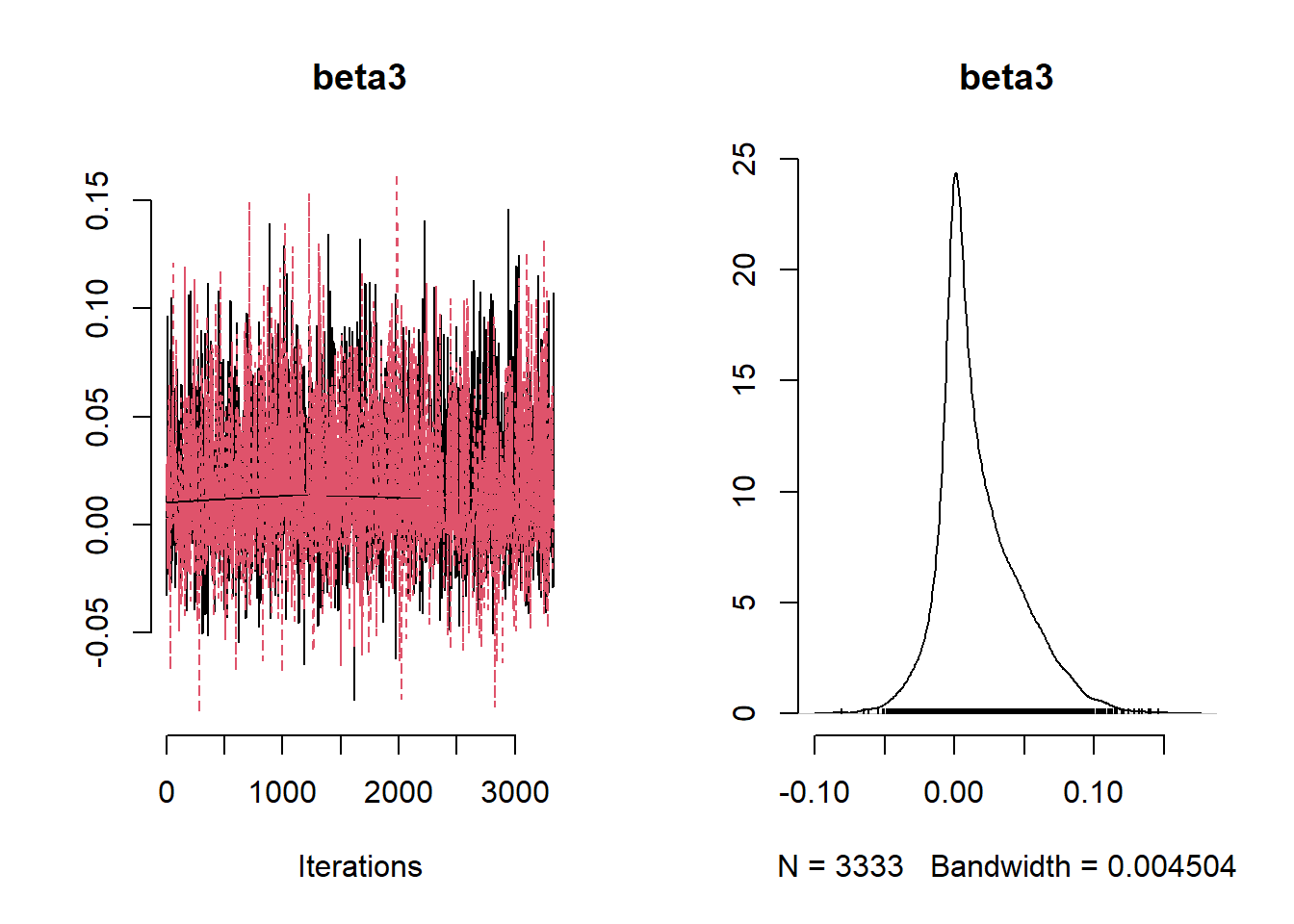
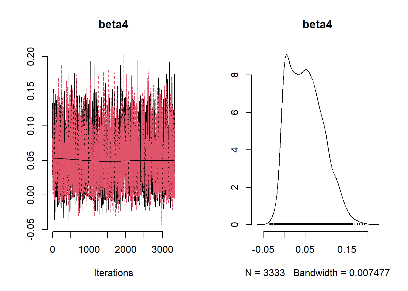
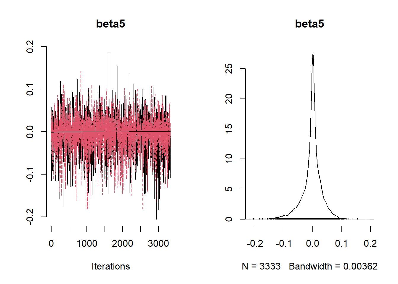
beta_var  <- paste0("beta[", 1:ncol(X), "]")
post_summary_hs <- mcmc.out.hs$summary$all.chains |> as.data.frame()
post_summary_hs <- post_summary_hs[beta_var,]

post_summary_hs$variable <- colnames(X)

ggplot(post_summary_hs,
       aes(x = variable)) +
  geom_pointrange(aes(y = Mean, ymin =`95%CI_low`, ymax =`95%CI_upp`)) +
  geom_hline(yintercept = 0) +
  theme_classic() + theme(axis.text.x = element_text(angle = 90, vjust = 0.5, hjust=1))