Chapter 11 Modelling temporal data: time series analysis and forecasting
The chapter contains the theory required for handling time series data. The reader will have gained an understanding of the following topics:
- that a temporal process consists of both low and high frequency components, the former playing a key role in determining long-term trends while the latter may be associated with shorter-term changes;
- techniques for the exploratory analysis of the data generated by the temporal process, including the ACF (correlogram) and PACF (periodogram);
- models for irregular (high frequency) components after the regular components (trend) have been removed;
- methods for forecasting, including exponential smoothing and ARIMA modelling;
- state space modelling approach, which sits naturally within a Bayesian setting and provides a general framework within which a wide class of models, including many classical time series models, can be expressed.
Example 11.1 Ground level ozone concentrations
Ozone is a colorless gas produced through a combination of photochemistry, sunlight, high temperatures, oxides of nitrogen, NO\(_x\),
emitted by motor vehicles. Levels are especially high during morning and evening commute hours
in urban areas. It is one of the criteria pollutants regulated by the US Clean Air Act (1970)
because of a substantial body of literature that shows a strong association with human morbidity, notably respiratory diseases such as
asthma, emphysema, and chronic obstructive pulmonary disorder (COPD) (EPA, 2005). Periods of high ozone concentrations can lead to acute asthma attacks leading to increased numbers of deaths, hospital admissions, and school absences. High levels of ozone concentrations can also lead to reduced
lung capacity.
Let’s start by loading the daily and hourly data for one site.
library(ggplot2)

# Load data for one site
site_daily <- read.csv("data/ozone/LA_ozone_daily.csv", header = TRUE)

# change the format of the date column
site_daily$date <- as.Date(site_daily$date, "%m/%d/%Y")

# load hourly data from that same site
site_hourly <- read.csv("data/ozone/LA_ozone_hourly.csv", header = TRUE)
The following plot shows daily concentrations of ozone measured at sites located in the geographical region of Los Angeles, California. Clear seasonal patterns can be observed due to the higher temperatures in summer.
# Plot daily data
ggplot(data = site_daily) +
  geom_line(aes(x = date, y = max.ozone, group = 1)) +
  # draw a line at the first data
  geom_vline(xintercept = as.Date("2013-01-01"), color = "grey") +
  # 8 hour regulatory standard of 0.075 (ppm)
  geom_hline(yintercept = 0.075, color = "grey") +
  xlab("Day in 2013 at Los Angeles Site 060379033") +
  ylab("Max Daily 8hr Ozone Level (ppm)") + theme_classic()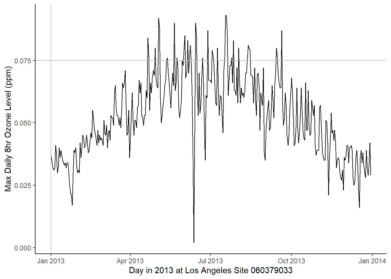
And the next plot depicts the same series at the hourly level, but restricted to the so-called `ozone season’, which is taken to be May 1 – Sep 30. Here a clear 24-hour daily cycle can be seen along with a period of missing data. The latter is likely due to the monitoring systems being checked each night by the injection of a calibrated sample of air. If the instrument reports the ozone incorrectly, an alert is sounded and that instrument is taken off-line until it is repaired. This can lead to gaps in the series, as seen around hour 1100.
# Plot hourly data
ggplot(data = site_hourly,) +
  geom_line(aes(x = time, y = ozone, group = 1)) +
  geom_vline(xintercept = 1, color = "grey") +
   # 8 hour regulatory standard of 0.075 (ppm).
  geom_hline(yintercept = 0.075, color = "grey") +
  xlab("Hour in 2013's ozone season") +
  ylab("Hourly Ozone Concentration (ppm)") +  theme_classic()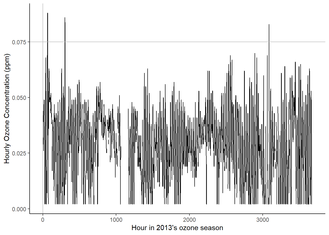
Example 11.2 Low-pass filtering of ozone levels using the moving average
We use the Ozone data of example 11.1 to look at moving averages of daily as done for carbon monoxide in example 11.3 discussed in the book.
For this example we will use the TTR package (Technical Trading Rules). This allow us to manipulate objects like time series for forecasting.
library(TTR)
# Load daily data
site_daily <- read.csv("data/ozone/LA_ozone_daily.csv", header = TRUE)
# add an identifier column for each day in the sample
site_daily$day <- 1:nrow(site_daily)
# Add loess smooth
# Single day moving average
ozone.loess <- loess(max.ozone ~ day, span = 0.75, data = site_daily[,c("max.ozone", "day")])
ozone.predict <- predict(ozone.loess, data.frame(day = 1:nrow(site_daily)))
ozone.predict_df <- data.frame(day = 1:nrow(site_daily),
ozone.prediction = ozone.predict)
plot_SMA1 <- ggplot(data = site_daily) +
geom_line(aes(x = day, y = max.ozone, group = 1)) +
geom_line(data = ozone.predict_df, aes(x = day, y = ozone.predict)) +
xlab("Day in 2013 at LA Site 060379033") +
ylab("Ozone Level (ppm)") +
ggtitle("Single day") +
theme_classic()
# Three day moving average
ozone_SMA3 <- data.frame(sma = SMA(site_daily$max.ozone, n = 3),
day = 1:nrow(site_daily))
plot_SMA3 <- ggplot(data = ozone_SMA3) +
geom_line(aes(x = day, y = sma, group = 1)) +
geom_line(data = ozone.predict_df, aes(x = day, y = ozone.predict)) +
xlab("Day in 2013 at LA Site 060379033") +
ylab("Ozone Level (ppm)") +
ggtitle("Three days") +
theme_classic()
# Six day moving average
ozone_SMA6 <- data.frame(sma = SMA(site_daily$max.ozone, n = 6),
day = 1:nrow(site_daily))
plot_SMA6 <- ggplot(data = ozone_SMA6) +
geom_line(aes(x = day, y = sma, group = 1)) +
geom_line(data = ozone.predict_df, aes(x = day, y = ozone.predict)) +
xlab("Day in 2013 at LA Site 060379033") +
ylab("Ozone Level (ppm)") +
ggtitle("Six days") +
theme_classic()
# Twelve day moving average
ozone_SMA12 <- data.frame(sma = SMA(site_daily$max.ozone, n = 12),
day = 1:nrow(site_daily))
plot_SMA12 <- ggplot(data = ozone_SMA12) +
geom_line(aes(x = day, y = sma, group = 1)) +
geom_line(data = ozone.predict_df, aes(x = day, y = ozone.predict)) +
xlab("Day in 2013 at LA Site 060379033") +
ylab("Ozone Level (ppm)") +
ggtitle("Twelve days") +
theme_classic()
cowplot::plot_grid(plot_SMA1, plot_SMA3, plot_SMA6, plot_SMA12, labels = "auto")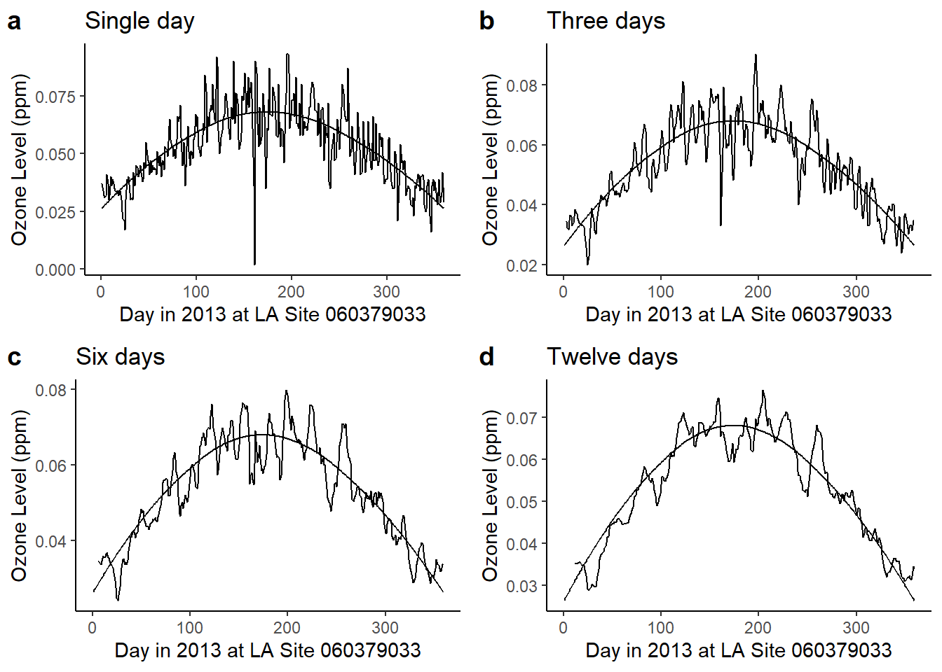
Example 11.12 Forecasting ozone levels
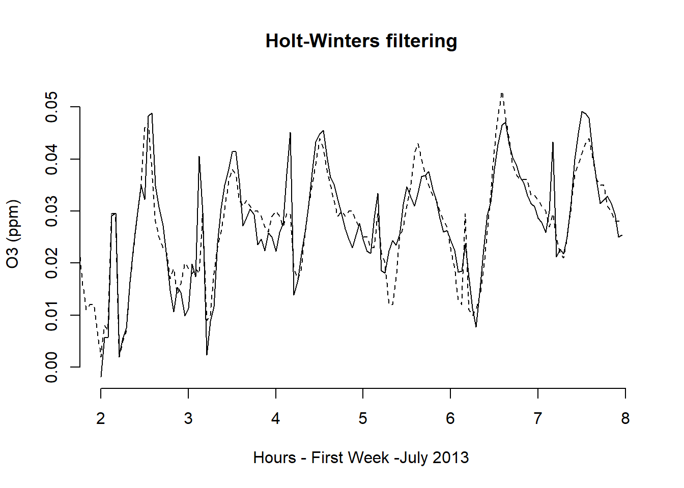
We return to Example 11.1 with the objective of forecasting ozone concentrations for the next twenty-four hours. These forecasts are based on measured concentrations in Los Angeles from the first week of July 2013. We first fit the Holt – Winters model and see the results in the first panel of the next Figure. The plot that follows shows the twenty-four-hour ahead forecast on day eight.\
library(TTR)
library(forecast)
# Load hourly data for site 060379033
site_hourly <- read.csv("data/ozone/LA_ozone_hourly.csv", header = TRUE)
# one night hour per day missing for instrument calibration - imputed for simplicity
imputeNA <- mean(site_hourly$ozone, na.rm = TRUE)
site_hourly$ozone[is.na(site_hourly$ozone)] <- imputeNA
# Select the first seven days in july
# days_pattern contains the dates for the first seven days
days_pattern <- paste0("^2013070", 1:7, collapse="|")
# select all the rows that follow that pattern using grepl
july_seven_days <- site_hourly[grepl(days_pattern, site_hourly$datetime),]
july_seven_days$hours <- 1:nrow(july_seven_days)
# Holt-Winters model fitting
# Turn this into a time series object to use Holt-Winters forecast
level_ts <- ts(july_seven_days$ozone,
frequency = 24,
start = c(1))
ozone_forecast <- HoltWinters(level_ts)
# Plot using the default function
plot(ozone_forecast,
xlab = "Hours - First Week -July 2013",
ylab = "O3 (ppm)",
col.predicted = 1,
col = "black",
bty = "n",
lty = 2
)
# Holt- Winters 24 ahead forast on Day 8
# no need to specify Holt-Winters forecast as the object is already HoltWinters class
ozoneforecast_day8 <- forecast(ozone_forecast, h=24)

# Plot using default function
plot(ozoneforecast_day8, bty = "n")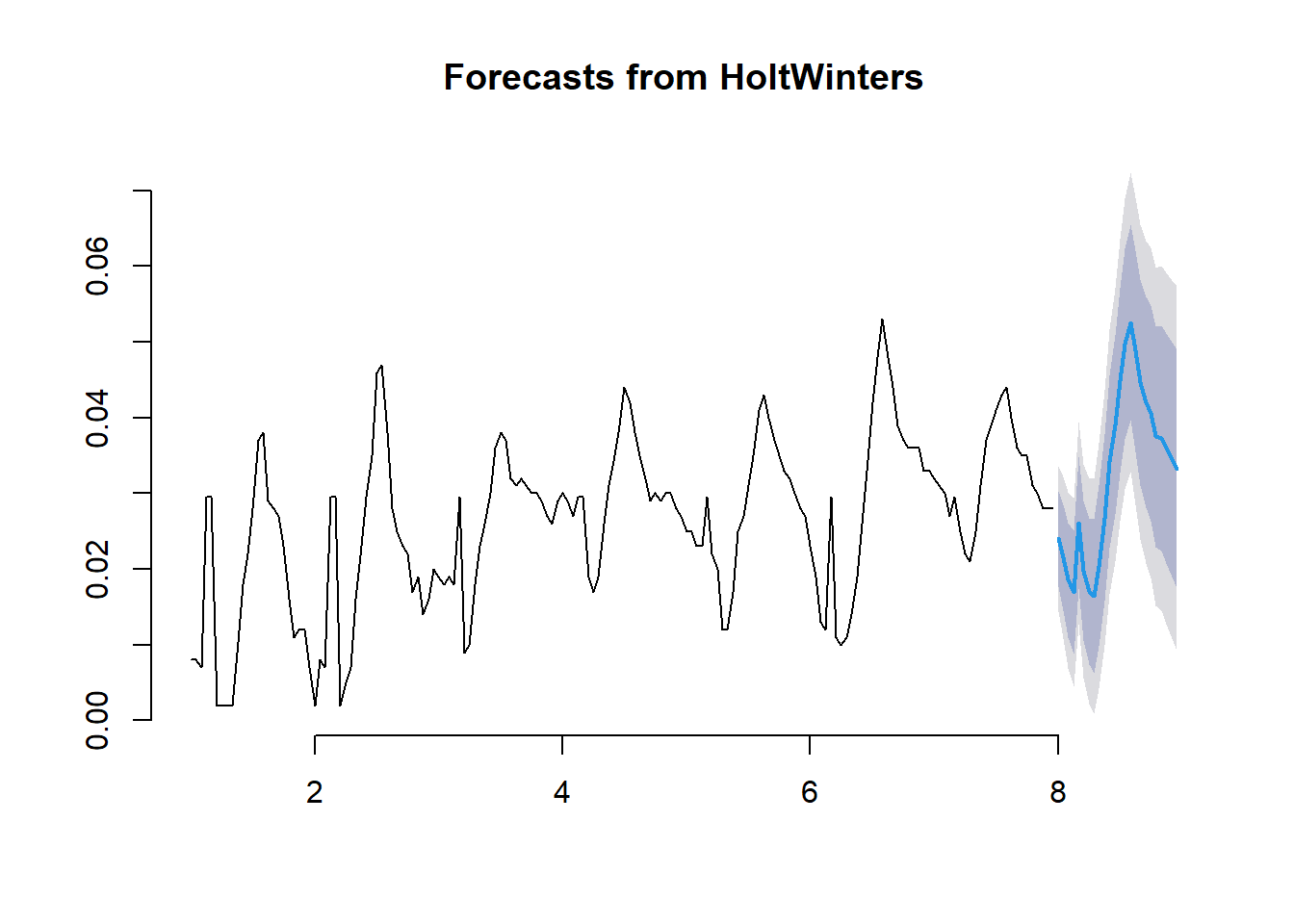
Example 11.13 Forecasting volcanic ash
Volcanic ash is not a substance that is commonly encountered in
environmental epidemiology, however it can be widely distributed by winds
and it can be a significant health hazard. A study
of the Mount St. Helens volcanic eruption in May and June 1980 reports thirty-five deaths due to the
initial blast and landslide. Others are reported to have died from asphyxiation from
ash inhalation (Baxter et al., 1981). The respirable portion of the ash was found to contain a small percentage of crystalline free silica, a potential pneumoconiosis hazard, and a number of acute health effects were found in those visiting emergency rooms including asthma, bronchitis
and ash-related eye problems.
The data in this example consists of atmospheric levels of volcanic ash from 1500AD to 2000AD.
library(ggplot2)
library(forecast)
library(TTR)

# Load volcano dust data
## REVIEW: Data source: Hyndman, R.J.  Time Series Data Library, http://data.is/TSDLdemo
# Data cover the period from 1500AD to 2000AD
volcano_dust <-
  scan("https://robjhyndman.com/tsdldata/annual/dvi.dat", skip = 1)
The following figure shows the plot of the original time series.
# Turn data into data frame to plot it in ggplot
volcano_dust_df <- data.frame(year = 1500:(1500+length(volcano_dust)-1),
                              dust = volcano_dust)

ggplot(data = volcano_dust_df) +
  geom_line(aes(x = year, y = dust, group = 1)) +
  xlab("Year") +
  ylab("Atmospheric levels of volcanic ash") + theme_classic()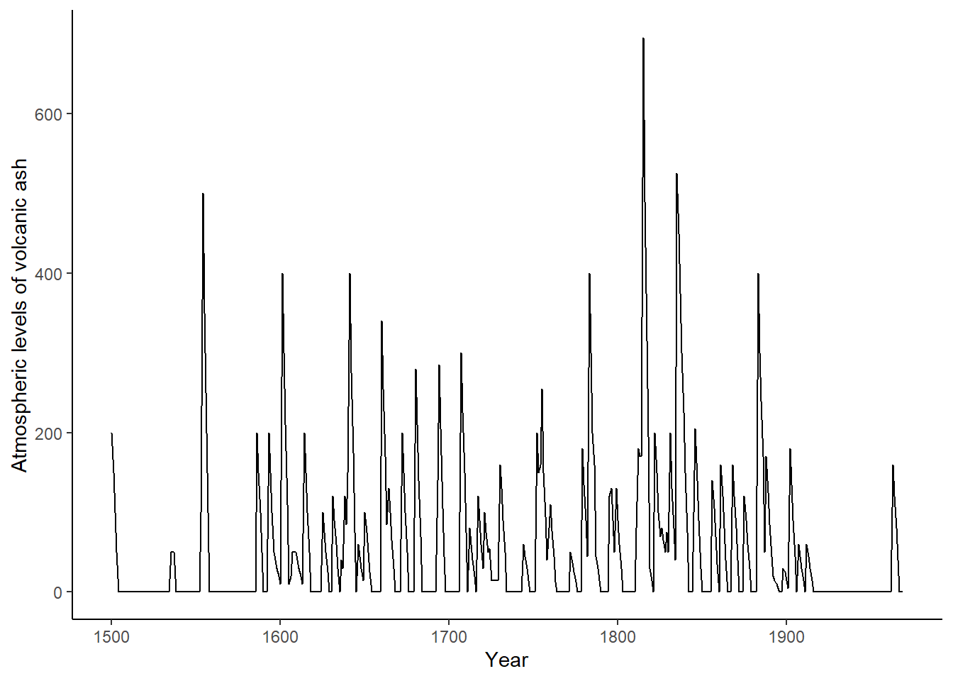
From the plot of the time series a complex pattern can be seen which is the result of eruptions occurring at random times. The large spikes suggest the possibility of moving average components, this is a way that the ARMA process has of incorporating shocks that abate over the period following their occurrence.
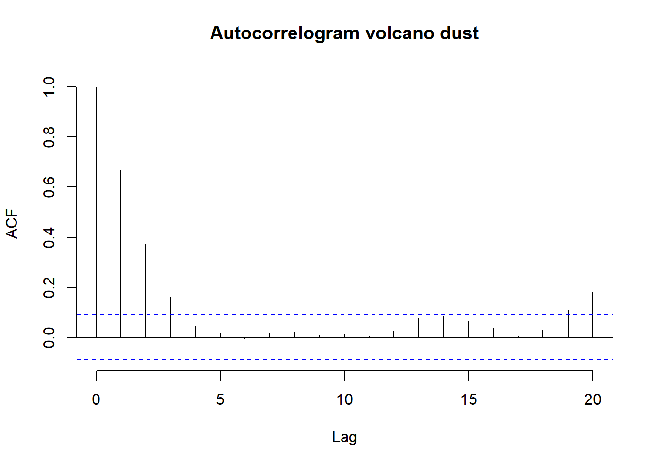
There are no obvious regular components in the series that would induce autocorrelation, so we turn to analysis of the ACF and PACF.
# convert data into a time series object
volcano_dust_series <- ts(volcano_dust, start = c(1500))
# Compute autocorrelogram with max lag 20
acf(
  volcano_dust_series,
  lag.max = 20,
  bty = "n",
  main = "Autocorrelogram volcano dust"
)
# Compute the partial autocorrelogram with max lag 20
pacf(
  volcano_dust_series,
  lag.max = 20,
  bty = "n",
  main = "Partial autocorrelogram volcano dust"
)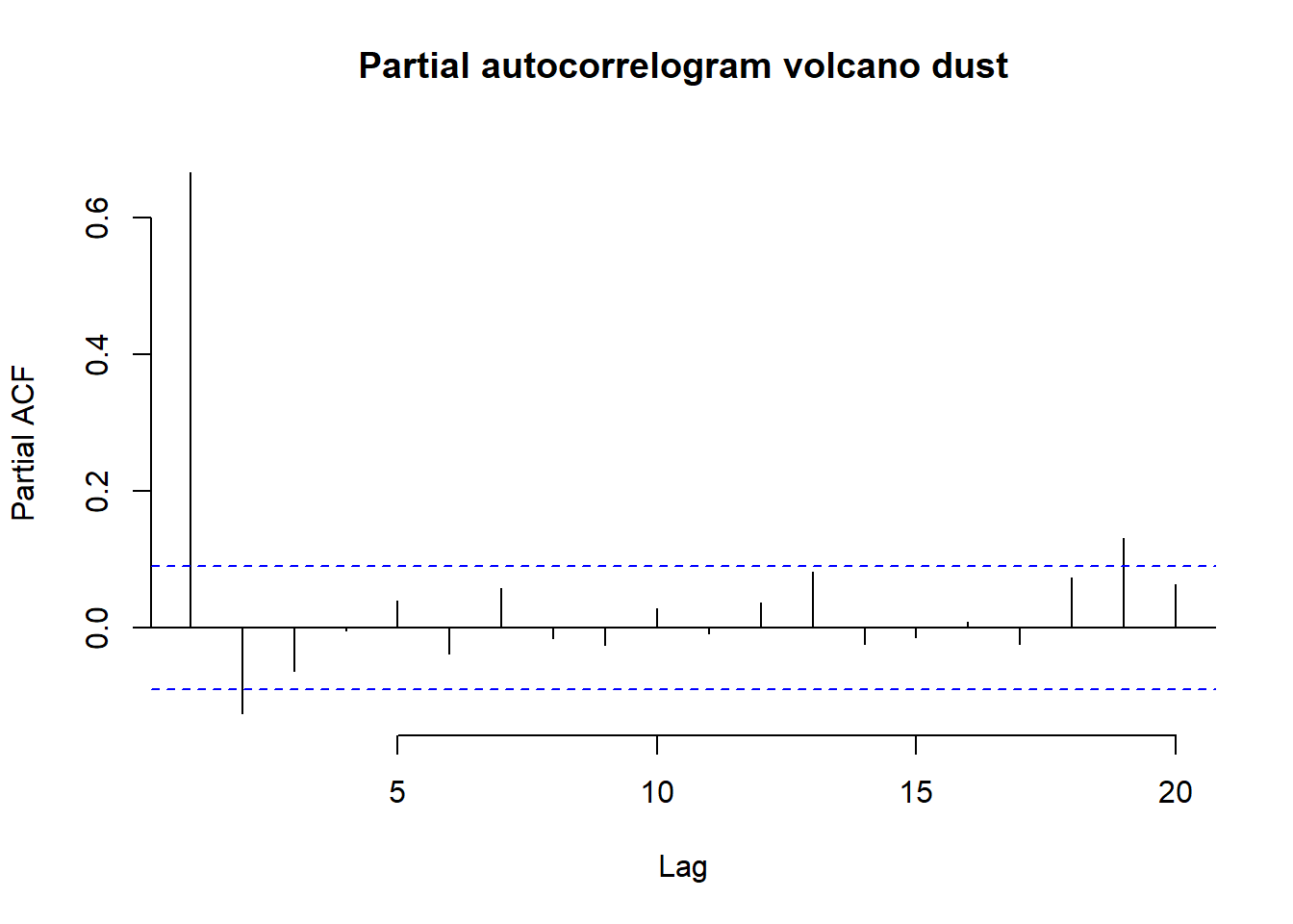
The correlogram is the first panel and it points to a significant autocorrelation at lag three and the possibility of an ARMA(0,3) model to capture the persistence in the ash level following a shock, and hence an MA(3) component or a mixture of an AR and MA model, might be considered. The PACF plot suggests a significant lag 2 effect, suggesting an ARMA(2,0) model.
The lack of obvious regular components, together with the correlogram plots, suggests the ARIMA approach differences may be used to achieve a
stationary process. The auto.arima function in the
R forecast library gives the following results (using the BIC criterion).
## Series: volcano_dust_series
## ARIMA(2,0,0) with non-zero mean
##
## Coefficients:
##          ar1      ar2     mean
##       0.7533  -0.1268  57.5274
## s.e.  0.0457   0.0458   8.5958
##
## sigma^2 = 4901:  log likelihood = -2662.54
## AIC=5333.09   AICc=5333.17   BIC=5349.7
# fitting the ARIMA(2,0,0) model
volcano_dust_arima <- arima(volcano_dust_series, order = c(2, 0, 0))
# forecast 31 years with the ARIMA(2,0,0) model
volcano_dust_forecast <- forecast(volcano_dust_arima, h = 31)
plot(volcano_dust_forecast, bty = "n")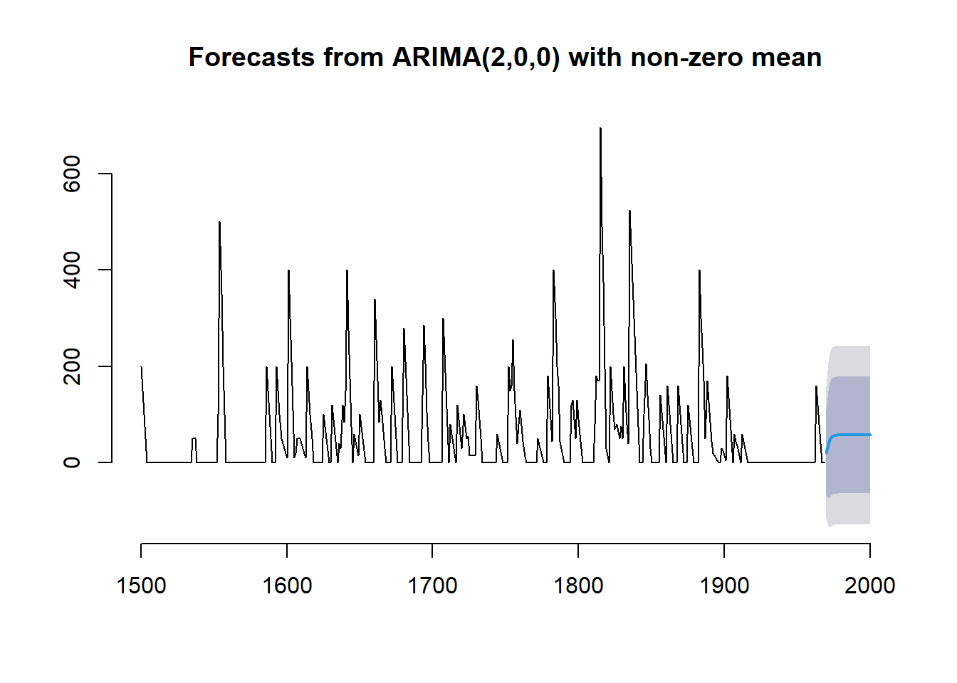
NOTE
The code for the implementation of DLMs in Stan and Nimble was developed by Paritosh Kumar Roy. This code and other more complex DLM structures are available through his github.
Example 11.17 Implementation of a dynamic linear model: UK ozone data
In this section we analyze the ozone concentration at one monitoring site in Aberdeen, UK from March to November 2017.
Nimble
library(coda)
library(dplyr)
#library(sf)
library(ggplot2)
library(nimble, warn.conflicts = FALSE)
library(nleqslv)
library(tidybayes)
library(tidyverse)

source("functions/FFBS_functions_nimble.R")

UK_ozone <- read.csv("data/ozone/uk_ozone_one_site.csv")
head(UK_ozone)
## ozone temp wind date
## 1 81.86627 2.433333 5.116667 2017-03-01
## 2 80.81055 2.754167 6.716667 2017-03-02
## 3 90.12082 2.716667 3.495833 2017-03-03
## 4 90.53892 5.320833 6.537500 2017-03-04
## 5 70.61635 4.920833 3.825000 2017-03-05
## 6 76.80751 2.479167 1.612500 2017-03-06Example11_16_O3_Nimble <- nimbleCode({
tau ~ T(dt(mu = 0, sigma = 1, df = 1), 0, Inf)
for (t in 1:Tt) {
Vt[t] <- tau ^ 2
}
for (j in 1:p) {
sqrt_Wt_diag[j] ~ T(dt(mu = 0, sigma = 1, df = 1), 0, Inf)
}
Wt[1:p, 1:p] <- nim_diag(x = sqrt_Wt_diag[1:p] ^ 2)
mt[1:p, 1] <- m0[1:p]
Ct[1:p, 1:p, 1] <- C0[1:p, 1:p]
for (t in 1:Tt) {
at[1:p, t] <- (Gt[1:p, 1:p] %*% mt[1:p, t])[1:p, 1]
Rt[1:p, 1:p, t] <-
Gt[1:p, 1:p] %*% Ct[1:p, 1:p, t] %*% t(Gt[1:p, 1:p]) + Wt[1:p, 1:p]
ft[t] <- (t(Ft[1:p, t]) %*% at[1:p, t])[1, 1]
Qt[t] <-
(t(Ft[1:p, t]) %*% Rt[1:p, 1:p, t] %*% Ft[1:p, t] + Vt[t])[1, 1]
yt[t] ~ dnorm(mean = ft[t], var = Qt[t])
At[1:p, t] <- (Rt[1:p, 1:p, t] %*% Ft[1:p, t])[1:p, 1] / Qt[t]
mt[1:p, t + 1] <- at[1:p, t] + (At[1:p, t] * (yt[t] - ft[t]))
Ct[1:p, 1:p, t + 1] <-
Rt[1:p, 1:p, t] - (At[1:p, t] %*% t(At[1:p, t])) * Qt[t]
}
theta[1:p, 1:(Tt + 1)] <-
nim_bsample(
mt = mt[1:p, 1:(Tt + 1)],
Ct = Ct[1:p, 1:p, 1:(Tt + 1)],
at = at[1:p, 1:Tt],
Gt = Gt[1:p, 1:p],
Rt = Rt[1:p, 1:p, 1:Tt]
)
})Time-varying level model
We first fit a time-varying level model such that,
\[\begin{aligned} Y_t &= F_t\theta_t + v_t, \qquad &v_t \sim \mathcal{N}(0, \tau^2) \\ \theta_t &= G_t\theta_{t-1} + \omega_t \qquad &\omega_t \sim \mathcal{N}(0, W^2) \end{aligned}\] For the time-varying mean model \(F_t = (1, \ wind_t, \ temp_t)\), and \(G_t = I_3\).
# Model specification
yt <- sqrt(UK_ozone$ozone)
temp <- UK_ozone$temp
wind <- UK_ozone$wind

Tt <- length(yt)
p <- 3 # (intercept, wind, temp)

Ft <- array(0, dim = c( p, Tt))
Ft[ 1,] <- 1
Ft[ 2,] <- (wind[1:Tt] - mean(wind[1:Tt])) / sd(wind[1:Tt])
Ft[ 3,] <- (temp[1:Tt] - mean(temp[1:Tt])) / sd(temp[1:Tt])

Gt <- diag(x = 1, nrow = p, ncol = p)
m0 <- c(mean(yt), 0, 0)
C0 <- diag(x = 1, nrow = p, ncol = p)


const_list <- list(Tt = Tt,
                   p = p)
dat_list <- list(
  yt = yt,
  Ft = Ft,
  Gt = Gt,
  m0 = m0,
  C0 = C0
)
init_list <- list(tau = 0.01, sqrt_Wt_diag = sqrt(rep(0.1, p)))

Rmodel <-
  nimbleModel(
    Example11_16_O3_Nimble,
    constants = const_list,
    data = dat_list,
    inits = init_list
  )
Rmodel$initializeInfo()
Rmodel$calculate()
Cmodel <- compileNimble(Rmodel, showCompilerOutput = FALSE)
conf <-
  configureMCMC(Rmodel, monitors = c("tau", "sqrt_Wt_diag", "theta", "ft"))

Rmcmc <- buildMCMC(conf)
Cmcmc <-
  compileNimble(
    Rmcmc,
    project = Cmodel,
    resetFunctions = TRUE,
    showCompilerOutput = FALSE
  )
niter <- 10000
nburnin <- 0.5 * niter
nthin <- 1
nchains <- 2
start_time <- Sys.time()
post_samples <-
  runMCMC(
    Cmcmc,
    niter = niter,
    nburnin = nburnin,
    thin = nthin,
    nchains = nchains,
    samplesAsCodaMCMC = TRUE
  )
end_time <- Sys.time()
run_time <- end_time - start_time
run_time
post_summary <- nimSummary(post_samples)
tidy_post_samples <- post_samples |> tidy_draws()
tidy_post_samples |>
dplyr::select(
.chain,
.iteration,
.draw,
'tau',
'sqrt_Wt_diag[1]',
'sqrt_Wt_diag[2]',
'sqrt_Wt_diag[3]'
) |>
gather(vars, value, -.chain, -.iteration, -.draw) |>
ggplot(aes(x = .iteration, y = value)) +
geom_path(aes(color = factor(.chain)), linewidth = 0.25,
show.legend = FALSE) +
facet_wrap( ~ vars, scales = "free", nrow = 2) +
theme_classic() +
theme(panel.grid = element_blank(),
strip.background = element_blank())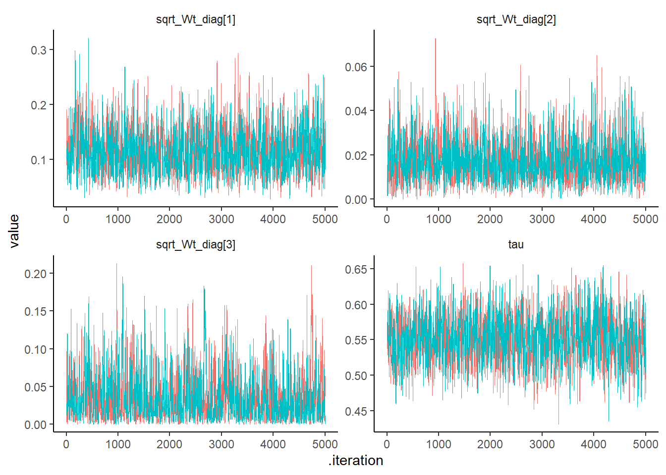
##                 post.mean post.sd  q2.5   q50 q97.5 f0    n.eff  Rhat
## tau                 0.550   0.033 0.487 0.551 0.614  1 1288.971 1.001
## sqrt_Wt_diag[1]     0.117   0.040 0.051 0.113 0.202  1 1161.622 1.001
## sqrt_Wt_diag[2]     0.017   0.009 0.004 0.016 0.039  1 1666.705 1.007
## sqrt_Wt_diag[3]     0.034   0.031 0.001 0.025 0.118  1  724.404 1.004
post_sum_theta <-
as.data.frame(post_summary) |> rownames_to_column() |>
filter(str_detect(rowname, "theta")) |>
dplyr::select(rowname, q2.5, q50, q97.5) |>
separate(rowname, into = c("x1", "x2"), sep = ",") |>
mutate(component = as.numeric(gsub(".*?([0-9]+).*", "\\1", x1))) |>
mutate(time = as.numeric(gsub(".*?([0-9]+).*", "\\1", x2))) |>
dplyr::select(component, time, q2.5, q50, q97.5)
ggplot(data = post_sum_theta, aes(x = time)) +
geom_ribbon(aes(ymin = q2.5, ymax = q97.5),
fill = "lightgray",
alpha = 0.7) +
geom_path(aes(y = q50), col = "blue", linewidth = 0.4) +
facet_wrap(
~ component,
nrow = 2,
scales = "free",
labeller = label_bquote(theta[.(component)])
) +
ylab("") + xlab("Time") +
theme_classic()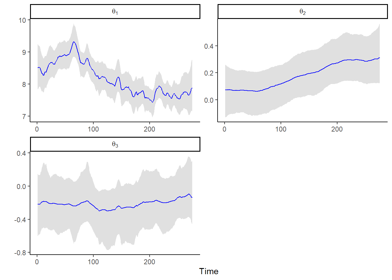
npsample <- floor((niter - nburnin)/nthin)
# str(tidy_post_samples)

Cnim_postfit_uoms <- compileNimble(nim_postfit_uoms, showCompilerOutput = FALSE)
## Compiling
## [Note] This may take a minute.
## [Note] Use 'showCompilerOutput = TRUE' to see C++ compilation details.post_tau <- tidy_post_samples$tau
post_sqrt_Wt_diag <-
tidy_post_samples |> dplyr::select(starts_with("sqrt_Wt_diag")) |>
as.matrix()|> unname()
post_ft_list <- lapply(1:(nchains*npsample), function(i) {
post_Vt <- post_tau[i]^2
post_Wt <- nim_diag(post_sqrt_Wt_diag[i,]^2)
post_ft <- Cnim_postfit_uoms(yt = dat_list$yt,
Ft = dat_list$Ft,
Vt = post_Vt,
Gt = dat_list$Gt,
Wt = post_Wt,
m0 = dat_list$m0,
C0 = dat_list$C0)
post_ft <- data.frame(ft = post_ft) |> mutate(time = row_number())
return(post_ft)
})
tidy_post_ft <- do.call("rbind", post_ft_list)
str(tidy_post_ft)## 'data.frame': 2750000 obs. of 2 variables:
## $ ft : num 10.67 10.06 9.77 8.48 9.02 ...
## $ time: int 1 2 3 4 5 6 7 8 9 10 ...## ft time
## 1 10.673309 1
## 2 10.055283 2
## 3 9.772315 3
## 4 8.479460 4
## 5 9.019850 5
## 6 8.055427 6## ft time
## 1 10.673309 1
## 2 10.055283 2
## 3 9.772315 3
## 4 8.479460 4
## 5 9.019850 5
## 6 8.055427 6post_sum_ft <- tidy_post_ft |> group_by(time) |>
summarise(post.mean = mean(ft),
post.sd = sd(ft),
q2.5 = quantile(ft, prob = 0.025),
q50 = quantile(ft, prob = 0.50),
q97.5 = quantile(ft, prob = 0.975)) |>
ungroup()
str(post_sum_ft)## tibble [275 × 6] (S3: tbl_df/tbl/data.frame)
## $ time : int [1:275] 1 2 3 4 5 6 7 8 9 10 ...
## $ post.mean: num [1:275] 8.14 8.96 8.95 8.66 9.2 ...
## $ post.sd : num [1:275] 2.296 1.277 1.139 0.789 0.761 ...
## $ q2.5 : Named num [1:275] 3.67 6.48 6.73 7.1 7.68 ...
## ..- attr(*, "names")= chr [1:275] "2.5%" "2.5%" "2.5%" "2.5%" ...
## $ q50 : Named num [1:275] 8.13 8.96 8.95 8.65 9.2 ...
## ..- attr(*, "names")= chr [1:275] "50%" "50%" "50%" "50%" ...
## $ q97.5 : Named num [1:275] 12.6 11.5 11.2 10.2 10.7 ...
## ..- attr(*, "names")= chr [1:275] "97.5%" "97.5%" "97.5%" "97.5%" ...## # A tibble: 6 × 6
## time post.mean post.sd q2.5 q50 q97.5
## <int> <dbl> <dbl> <dbl> <dbl> <dbl>
## 1 1 8.14 2.30 3.67 8.13 12.6
## 2 2 8.96 1.28 6.48 8.96 11.5
## 3 3 8.95 1.14 6.73 8.95 11.2
## 4 4 8.66 0.789 7.10 8.65 10.2
## 5 5 9.20 0.761 7.68 9.20 10.7
## 6 6 8.90 0.909 7.08 8.89 10.7ggplot(data = post_sum_ft, aes(x = time)) +
geom_ribbon(aes(ymin = q2.5,ymax = q97.5), fill = "lightgray") +
geom_path(aes(y = post.mean), linewidth = 0.25) +
geom_point(aes(y=yt), size = 0.25) +
ylab("Ozone Level (ppm)") +
xlab("Time") + ggtitle("Fitted values Ozone level UK") +
theme_classic()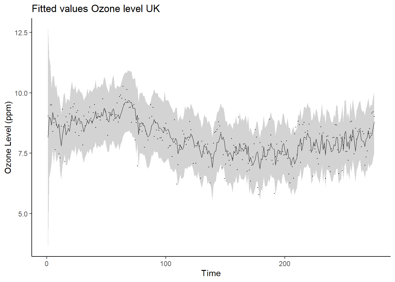

Trend model
In this case we include a trend then, \(F_t = (1, 0, \ wind_t, \ temp_t)\) and \(G_t = \begin{pmatrix} 1 & 1 \\ 0 & 1\end{pmatrix}\).
# Model specification
yt <- sqrt(UK_ozone$ozone)
temp <- UK_ozone$temp
wind <- UK_ozone$wind

Tt <- length(yt)
p <- 4 # (intercept, trend, wind, temp)

Ft <- array(0, dim = c( p, Tt))
Ft[1,] <- 1
Ft[2,] <- 0
Ft[3,] <- (wind[1:Tt] - mean(wind[1:Tt])) / sd(wind[1:Tt])
Ft[4,] <- (temp[1:Tt] - mean(temp[1:Tt])) / sd(temp[1:Tt])


Gt <- diag(x = 1, nrow = p, ncol = p)
Gt[1, 2] <- 1

m0 <- c(mean(yt), 0, 0, 0)
C0 <- diag(x = 1, nrow = p, ncol = p)

const_list <- list(Tt = Tt,
                   p = p)
dat_list <- list(
  yt = yt,
  Ft = Ft,
  Gt = Gt,
  m0 = m0,
  C0 = C0
)
init_list <- list(tau = 0.01, sqrt_Wt_diag = sqrt(rep(0.1, p)))

Rmodel <-
  nimbleModel(
    Example11_16_O3_Nimble,
    constants = const_list,
    data = dat_list,
    inits = init_list
  )
Rmodel$initializeInfo()
Rmodel$calculate()
Cmodel <- compileNimble(Rmodel, showCompilerOutput = FALSE)
conf <-
  configureMCMC(Rmodel, monitors = c("tau", "sqrt_Wt_diag", "theta", "ft"))

Rmcmc <- buildMCMC(conf)
Cmcmc <-
  compileNimble(
    Rmcmc,
    project = Cmodel,
    resetFunctions = TRUE,
    showCompilerOutput = FALSE
  )
niter <- 10000
nburnin <- 0.5 * niter
nthin <- 1
nchains <- 2
start_time <- Sys.time()
post_samples <-
  runMCMC(
    Cmcmc,
    niter = niter,
    nburnin = nburnin,
    thin = nthin,
    nchains = nchains,
    samplesAsCodaMCMC = TRUE
  )
end_time <- Sys.time()
run_time <- end_time - start_time
run_time
post_summary <- nimSummary(post_samples)
tidy_post_samples <- post_samples |> tidy_draws()
tidy_post_samples |>
dplyr::select(
.chain,
.iteration,
.draw,
'tau',
'sqrt_Wt_diag[1]',
'sqrt_Wt_diag[2]',
'sqrt_Wt_diag[3]',
'sqrt_Wt_diag[4]'
) |>
gather(vars, value, -.chain, -.iteration, -.draw) |>
ggplot(aes(x = .iteration, y = value)) +
geom_path(aes(color = factor(.chain)), linewidth = 0.25,
show.legend = FALSE) +
facet_wrap( ~ vars, scales = "free", nrow = 2) +
theme_classic() +
theme(panel.grid = element_blank(),
strip.background = element_blank())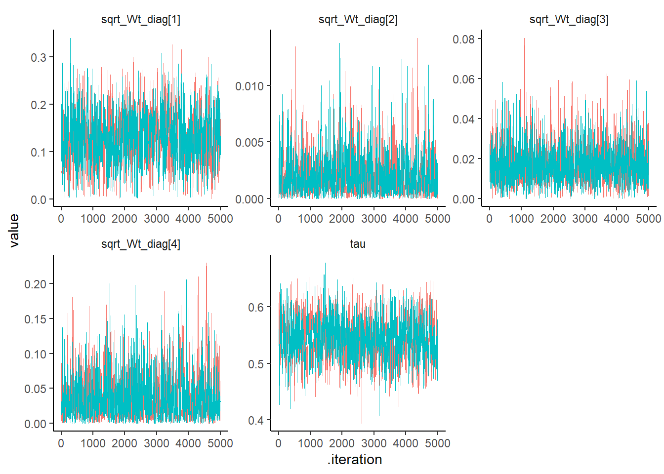
post_summary[c('tau',
               'sqrt_Wt_diag[1]',
               'sqrt_Wt_diag[2]',
               'sqrt_Wt_diag[3]',
               'sqrt_Wt_diag[4]'), ]
## post.mean post.sd q2.5 q50 q97.5 f0 n.eff Rhat
## tau 0.544 0.037 0.471 0.543 0.615 1 875.124 1.004
## sqrt_Wt_diag[1] 0.131 0.055 0.030 0.128 0.244 1 850.247 1.002
## sqrt_Wt_diag[2] 0.002 0.002 0.000 0.002 0.007 1 930.546 1.000
## sqrt_Wt_diag[3] 0.017 0.009 0.004 0.016 0.040 1 1694.931 1.009
## sqrt_Wt_diag[4] 0.036 0.032 0.001 0.027 0.120 1 1002.860 1.023post_sum_theta <-
as.data.frame(post_summary) |> rownames_to_column() |>
filter(str_detect(rowname, "theta")) |>
dplyr::select(rowname, q2.5, q50, q97.5) |>
separate(rowname, into = c("x1", "x2"), sep = ",") |>
mutate(component = as.numeric(gsub(".*?([0-9]+).*", "\\1", x1))) |>
mutate(time = as.numeric(gsub(".*?([0-9]+).*", "\\1", x2))) |>
dplyr::select(component, time, q2.5, q50, q97.5)
ggplot(data = post_sum_theta, aes(x = time)) +
geom_ribbon(aes(ymin = q2.5, ymax = q97.5),
fill = "lightgray",
alpha = 0.7) +
geom_path(aes(y = q50), col = "blue", linewidth = 0.4) +
facet_wrap(
~ component,
nrow = 2,
scales = "free",
labeller = label_bquote(theta[.(component)])
) +
ylab("") +
xlab("Time") +
theme_classic()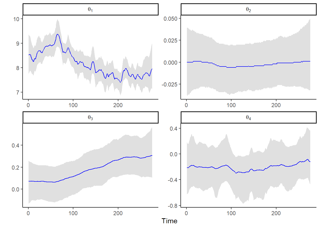
npsample <- floor((niter - nburnin)/nthin)

Cnim_postfit_uoms <- compileNimble(nim_postfit_uoms, showCompilerOutput = FALSE)
## Compiling
## [Note] This may take a minute.
## [Note] Use 'showCompilerOutput = TRUE' to see C++ compilation details.post_tau <- tidy_post_samples$tau
post_sqrt_Wt_diag <-
tidy_post_samples |> dplyr::select(starts_with("sqrt_Wt_diag")) |>
as.matrix()|> unname()
post_ft_list <- lapply(1:(nchains*npsample), function(i) {
post_Vt <- post_tau[i]^2
post_Wt <- nim_diag(post_sqrt_Wt_diag[i,]^2)
post_ft <- Cnim_postfit_uoms(yt = dat_list$yt,
Ft = dat_list$Ft,
Vt = post_Vt,
Gt = dat_list$Gt,
Wt = post_Wt,
m0 = dat_list$m0,
C0 = dat_list$C0)
post_ft <- data.frame(ft = post_ft) |> mutate(time = row_number())
return(post_ft)
})
tidy_post_ft <- do.call("rbind", post_ft_list)
## posterior summaries of ft
post_sum_ft <- tidy_post_ft |> group_by(time) |>
summarise(post.mean = mean(ft),
post.sd = sd(ft),
q2.5 = quantile(ft, prob = 0.025),
q50 = quantile(ft, prob = 0.50),
q97.5 = quantile(ft, prob = 0.975)) |>
ungroup()
ggplot(data = post_sum_ft, aes(x = time)) +
geom_ribbon(aes(ymin = q2.5,ymax = q97.5), fill = "lightgray") +
geom_path(aes(y = post.mean), size = 0.25) +
geom_point(aes(y=yt), size = 0.25) +
ylab("Ozone Level (ppm)") +
xlab("Time") + ggtitle("Fitted values Ozone level UK") +
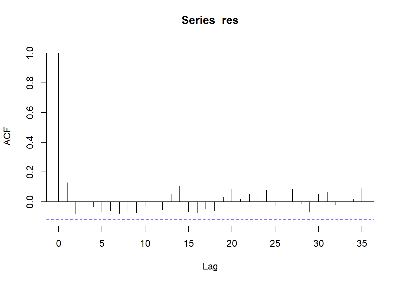
theme_classic()## Warning: Using `size` aesthetic for lines was deprecated
## in ggplot2 3.4.0.
## ℹ Please use `linewidth` instead.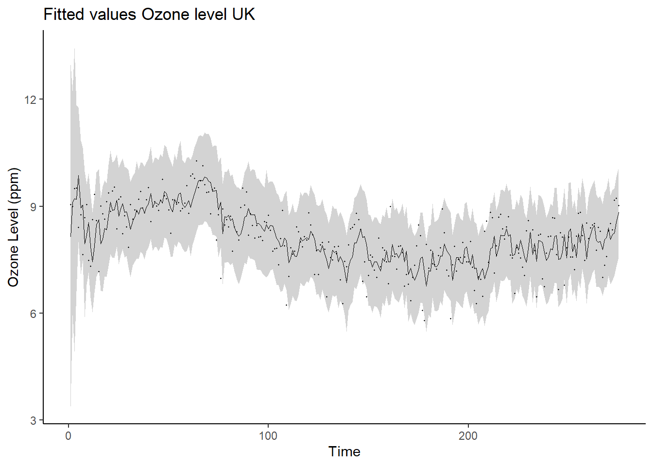
Stan
library(coda)
library(ggplot2)
library(gridExtra)
library(rstan)
library(tidyverse)

options(mc.cores = parallel::detectCores())
rstan_options(auto_write = TRUE)

# Load data for RW case
UK_ozone <- read.csv("data/ozone/uk_ozone_one_site.csv")
Time-varying level model
y <- sqrt(UK_ozone$ozone)
temp <- UK_ozone$temp
wind <- UK_ozone$wind

Tt <- length(y)
p <- 3 # (intercept, wind, temp)

Ft <- array(0, dim = c(Tt, p))
Ft[, 1] <- 1
Ft[, 2] <- (wind[1:Tt] - mean(wind[1:Tt])) / sd(wind[1:Tt])
Ft[, 3] <- (temp[1:Tt] - mean(temp[1:Tt])) / sd(temp[1:Tt])

Gt <- diag(x = 1, nrow = p, ncol = p)
m0 <- c(mean(y), 0, 0)
C0 <- diag(x = 1, nrow = p, ncol = p)

stan_data <- list(T = Tt, p = p, y = y, F = Ft, G = Gt, m0= m0, C0 = C0)
functions {
// FFBS for DLM with univariate observation equation and univariate system equation
array[] vector uoms_ffbs_rng(array[] real y, array[] vector F, matrix G, real V, matrix W, vector m0, matrix C0, int T, int p){
array[T] vector[p] theta;
array[T] vector[p] a;
array[T] matrix[p,p] R;
array[T] vector[p] m;
array[T] matrix[p,p] C;
// Kalman filtering
vector[p] mt = m0;
matrix[p,p] Ct = C0;
for(i in 1:T){
real ft;
real Qt;
vector[p] at;
matrix[p,p] Rt;
vector[p] At;
at = G * mt;
Rt = G * Ct * G' + W;
ft = F[i]' * at;
Qt = quad_form(Rt, F[i]) + V; //F[i]' * Rt * F[i] + V;
At = Rt * F[i] * inv(Qt);
mt = at + At * (y[i] - ft);
Ct = Rt - At * Qt * At';
//store for backward sampling
a[i] = at;
R[i] = Rt;
m[i] = mt;
C[i] = Ct;
}
// backward sampling
array[T-1] int ind = sort_indices_desc(linspaced_int_array(T-1,1,T-1));
theta[T] = multi_normal_rng(m[T], C[T]);
for(i in ind) {
matrix[p,p] Bt;
vector[p] ht;
matrix[p,p] Ht;
Bt = C[i] * G' * inverse(R[i+1]);
ht = m[i] + Bt * (theta[i+1] - a[i+1]);
Ht = C[i] - Bt * R[i+1] * Bt';
theta[i] = multi_normal_rng(ht, Ht);
}
return theta;
}
real uoms_dlm_ldensity(array[] real y, array[] vector F, matrix G, real V, matrix W, vector m0, matrix C0, int T, int p){
array[T+1] vector[p] a;
array[T+1] matrix[p, p] R;
array[T] real lldata;
a[1] = m0;
R[1] = C0;
for (i in 1:T) {
real u;
real Q;
real Qinv;
vector[p] A;
matrix[p, p] L;
u = y[i] - F[i]' * a[i];
Q = quad_form(R[i],F[i]) + V; //F[i]' * R[i] * F[i] + V;
Qinv = inv(Q); //
A = G * R[i] * F[i] * Qinv;
L = G - A * F[i]';
//lldata[i] = -0.5 * (log(2 * pi()) + log(Q) + Qinv*square(u));
lldata[i] = normal_lpdf(u | 0, sqrt(Q)); // univariate
a[i+1] = G * a[i] + A * u;
R[i+1] = G * R[i] * L' + W;
}
return sum(lldata);
}
array[] real uoms_dlm_one_step_ahead_rng(array[] real y, array[] vector F, matrix G, real V, matrix W, vector m0, matrix C0, int T, int p){
array[T] real yfit;
array[T+1] vector[p] a;
array[T+1] matrix[p, p] R;
array[T] real lldata;
a[1] = m0;
R[1] = C0;
for (i in 1:T) {
real u;
real Q;
real Qinv;
vector[p] A;
matrix[p, p] L;
u = y[i] - F[i]' * a[i];
Q = quad_form(R[i],F[i]) + V; //F[i]' * R[i] * F[i] + V;
Qinv = inv(Q); //
A = G * R[i] * F[i] * Qinv;
L = G - A * F[i]';
yfit[i] = normal_rng(F[i]' * a[i], sqrt(Q)); // univariate
a[i+1] = G * a[i] + A * u;
R[i+1] = G * R[i] * L' + W;
}
return yfit;
}
}
data{
int T;
int p;
array[T] real y;
array[T] vector[p] F;
matrix[p, p] G;
vector[p] m0;
cov_matrix[p] C0;
}
parameters{
real<lower=0> tau;
vector<lower=0>[p] sqrt_W_diag;
}
model {
real V = square(tau);
matrix[p, p] W = diag_matrix(square(sqrt_W_diag));
tau ~ std_normal();
sqrt_W_diag ~ std_normal();
target += uoms_dlm_ldensity(y, F, G, V, W, m0, C0, T, p);
}
generated quantities{
array[T] vector[p] theta;
array[T] real yfit;
real V = square(tau);
matrix[p, p] W = diag_matrix(square(sqrt_W_diag));
theta = uoms_ffbs_rng(y, F, G, V, W, m0, C0, T, p);
yfit = uoms_dlm_one_step_ahead_rng(y, F, G, V, W, m0, C0, T, p);
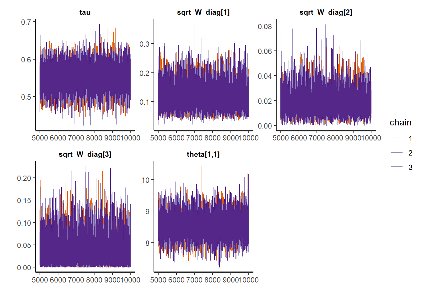
}Example11_16_UK_Stan <- stan(
file = "functions/Example11_16_UK.stan",
data = stan_data,
warmup = 5000,
iter = 10000,
chains = 3,
include = TRUE
)
rstan::traceplot(Example11_16_UK_Stan,
                 pars = paste0("theta[", sample.int(Tt, size = 4, replace = FALSE), ",1]"))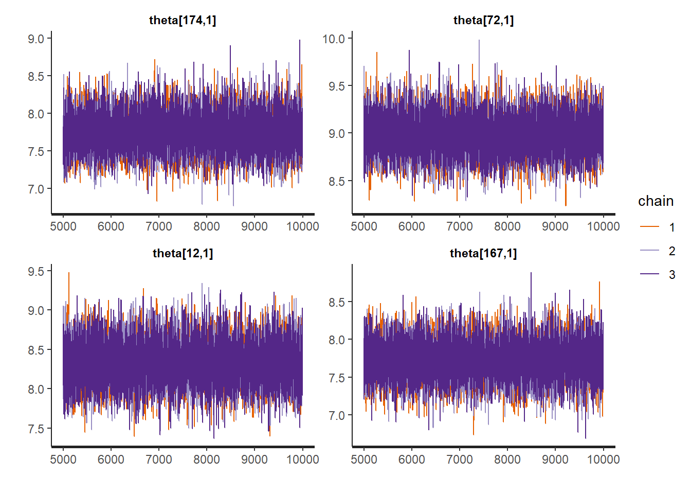
rstan::traceplot(Example11_16_UK_Stan,
                 pars = paste0("theta[", sample.int(Tt, size = 4, replace = FALSE), ",2]"))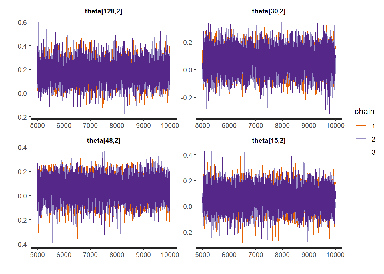
rstan::traceplot(Example11_16_UK_Stan,
                 pars = paste0("theta[", sample.int(Tt, size = 4, replace = FALSE), ",3]"))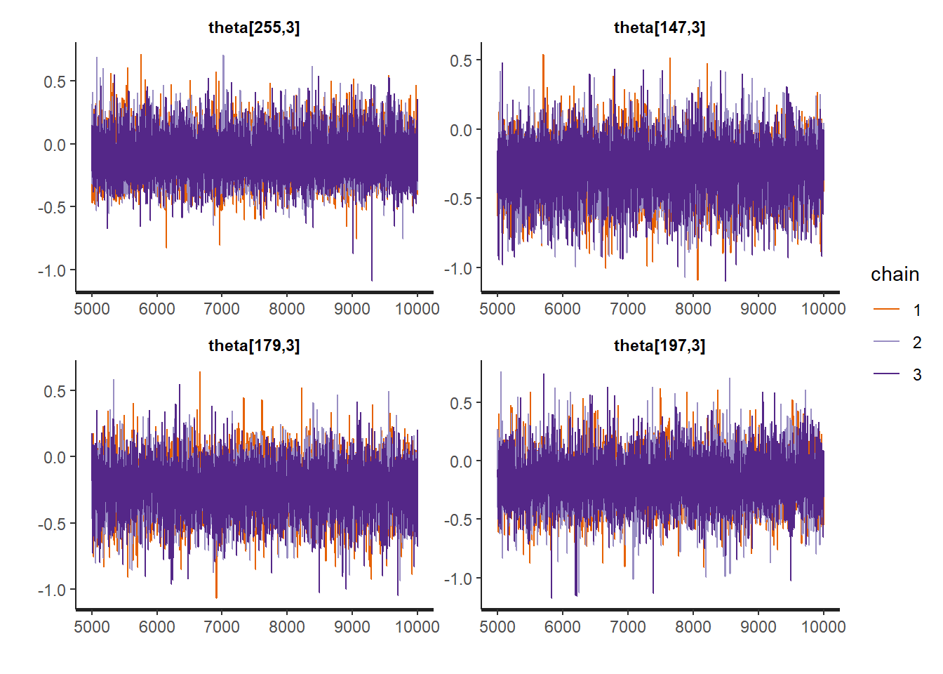
fixedpars_summary <-
  summary(Example11_16_UK_Stan, pars = c("tau", "sqrt_W_diag"))$summary
fixedpars_summary
## mean se_mean sd 2.5% 25%
## tau 0.54952783 3.456478e-04 0.033200616 0.483950759 0.52724045
## sqrt_W_diag[1] 0.11879062 4.682828e-04 0.042765301 0.051417741 0.08668241
## sqrt_W_diag[2] 0.01702899 8.180045e-05 0.008928214 0.003498400 0.01079707
## sqrt_W_diag[3] 0.03420662 3.088344e-04 0.030751202 0.001145905 0.01123936
## 50% 75% 97.5% n_eff Rhat
## tau 0.54963949 0.57140419 0.61408371 9226.237 1.0003090
## sqrt_W_diag[1] 0.11341398 0.14535262 0.21426583 8340.013 1.0000506
## sqrt_W_diag[2] 0.01557511 0.02165377 0.03841738 11912.906 0.9999899
## sqrt_W_diag[3] 0.02543997 0.04824451 0.11442124 9914.543 1.0001423theta_summary <-
summary(Example11_16_UK_Stan, pars = c("theta"))$summary
yfit_summary <-
summary(Example11_16_UK_Stan, pars = c("yfit"))$summary
p1 <- data.frame(theta_summary) |>
rownames_to_column() |>
filter(rowname %in% paste0("theta[", 1:Tt, ",1]")) |>
mutate(date = as.Date(UK_ozone$date[1:Tt])) |>
ggplot(aes(x = date, group = 1)) +
geom_path(aes(y = mean), color = "blue", linewidth = 0.6) +
geom_ribbon(aes(ymin = X2.5., ymax = X97.5.),
alpha = 0.25,
col = "lightgray") +
ggtitle("Intercept") + theme_classic() +
theme(plot.title = element_text(hjust = 0.5))
p2 <- data.frame(theta_summary) |>
rownames_to_column() |>
filter(rowname %in% paste0("theta[", 1:Tt, ",2]")) |>
mutate(date = as.Date(UK_ozone$date[1:Tt])) |>
ggplot(aes(x = date)) +
geom_path(aes(y = mean), color = "blue", linewidth = 0.6) +
geom_ribbon(aes(ymin = X2.5., ymax = X97.5.),
alpha = 0.25,
col = "lightgray") +
ggtitle("Wind") + theme_classic() +
theme(plot.title = element_text(hjust = 0.5))
p3 <- data.frame(theta_summary) |>
rownames_to_column() |>
filter(rowname %in% paste0("theta[", 1:Tt, ",3]")) |>
mutate(date = as.Date(UK_ozone$date[1:Tt])) |>
ggplot(aes(x = date)) +
geom_path(aes(y = mean), color = "blue", linewidth = 0.6) +
geom_ribbon(aes(ymin = X2.5., ymax = X97.5.),
alpha = 0.25,
col = "lightgray") +
ggtitle("Temperature") + theme_classic() +
theme(plot.title = element_text(hjust = 0.5))
grid.arrange(p1,p2,p3, ncol = 2)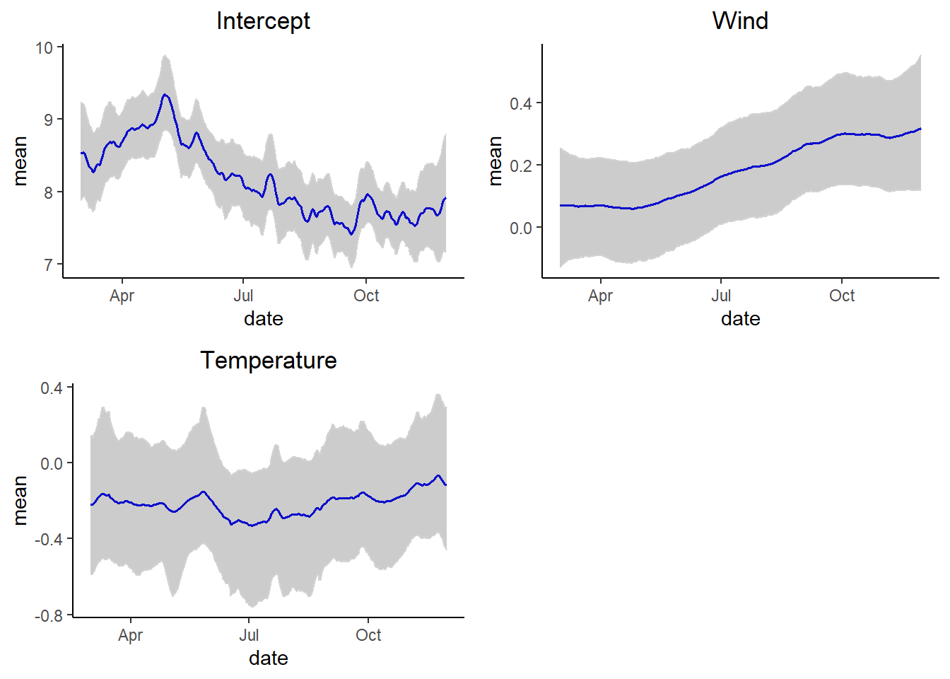
# Fitted values
yfit_summary_dt <- data.frame(yfit_summary) |>
  rownames_to_column() |>
  mutate(time = as.numeric(gsub(".*?([0-9]+).*", "\\1", rowname)))

ggplot(yfit_summary_dt, aes(x = time)) +
  geom_ribbon(aes(ymin = X2.5., ymax = X97.5.),
              alpha = 0.25,
              col = "gray99") +
  geom_point(aes(y = y)) +
  geom_path(aes(y = mean), linewidth = 0.1, size = 1) +
 ylab("Ozone Level (ppm)") +
  xlab("Time") + ggtitle("Fitted values Ozone level UK") +
  theme_classic()
## Warning: Using `size` aesthetic for lines was deprecated in ggplot2 3.4.0.
## ℹ Please use `linewidth` instead.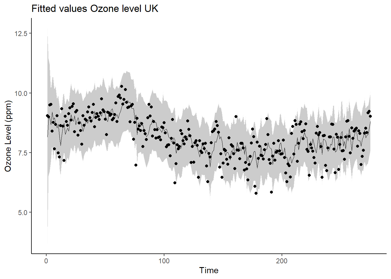
Trend model
y <- sqrt(UK_ozone$ozone)
temp <- UK_ozone$temp
wind <- UK_ozone$wind

Tt <- length(y)
p <- 4 # (intercept, trend, wind, temp)

Ft <- array(0, dim = c(Tt, p))
Ft[, 1] <- 1
Ft[, 2] <- 0
Ft[, 3] <- (wind[1:Tt] - mean(wind[1:Tt])) / sd(wind[1:Tt])
Ft[, 4] <- (temp[1:Tt] - mean(temp[1:Tt])) / sd(temp[1:Tt])

Gt <- diag(x = 1, nrow = p, ncol = p)
Gt[1, 2] <- 1


m0 <- c(mean(y), 0, 0, 0)
C0 <- diag(x = 1, nrow = p, ncol = p)

stan_data_trend <- list(
  T = Tt,
  p = p,
  y = y,
  F = Ft,
  G = Gt,
  m0 = m0,
  C0 = C0
)

Example11_16_UK_trend_Stan  <- stan(
  file = "functions/Example11_16_UK.stan",
  data = stan_data_trend,
  warmup = 5000,
  iter = 10000,
  chains = 3,
  include = TRUE
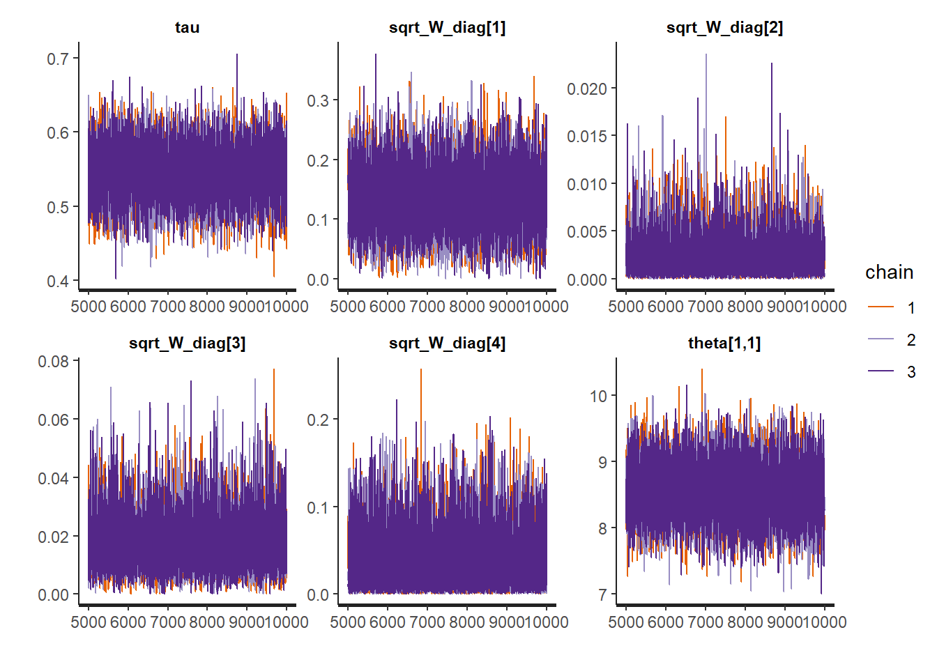
)
rstan::traceplot(Example11_16_UK_trend_Stan,
                 pars = paste0("theta[", sample.int(Tt, size = 4, replace = FALSE), ",1]"))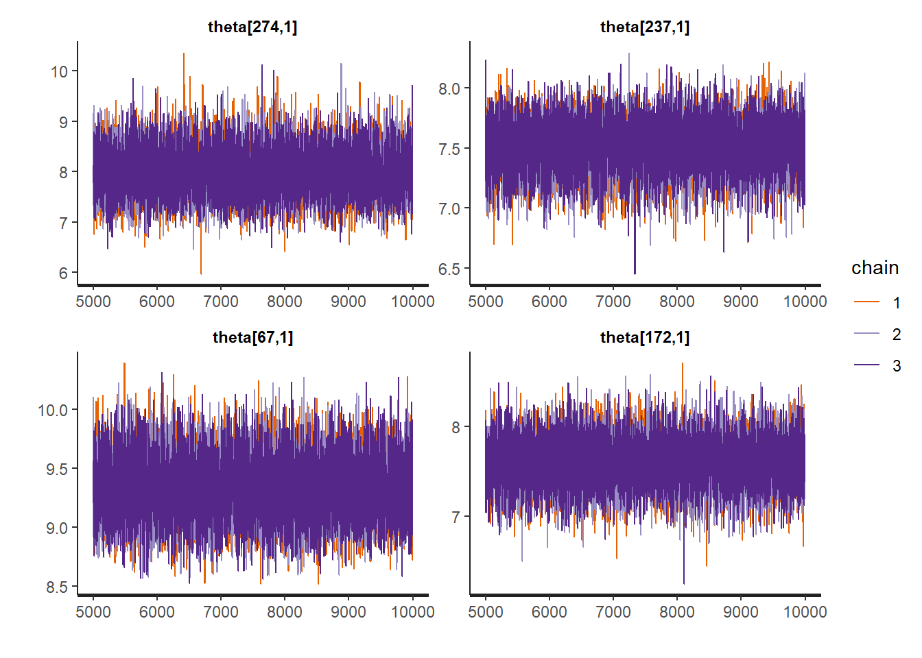
rstan::traceplot(Example11_16_UK_trend_Stan,
                 pars = paste0("theta[", sample.int(Tt, size = 4, replace = FALSE), ",2]"))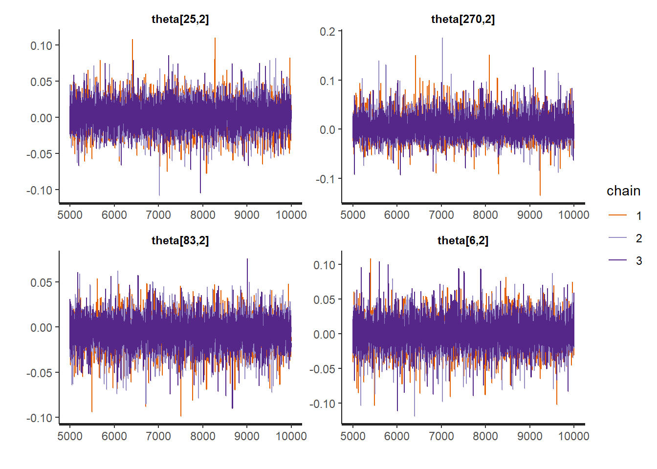
rstan::traceplot(Example11_16_UK_trend_Stan,
                 pars = paste0("theta[", sample.int(Tt, size = 4, replace = FALSE), ",3]"))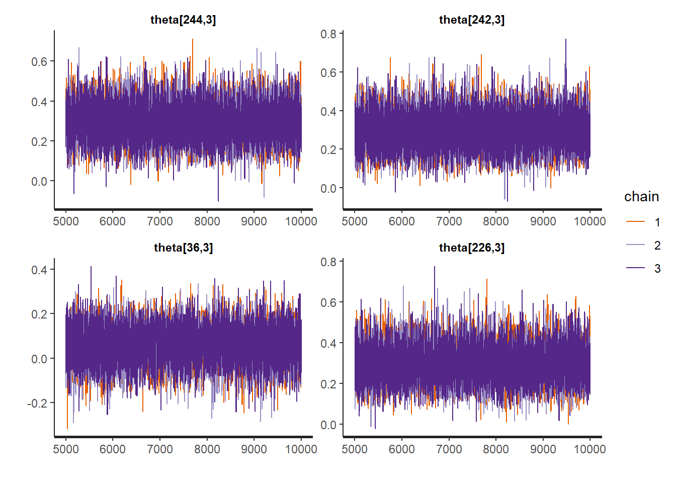
rstan::traceplot(Example11_16_UK_trend_Stan,
                 pars = paste0("theta[", sample.int(Tt, size = 4, replace = FALSE), ",4]"))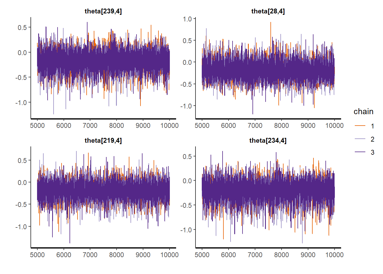
fixedpars_summary <-
  summary(Example11_16_UK_trend_Stan, pars = c("tau", "sqrt_W_diag"))$summary
fixedpars_summary
## mean se_mean sd 2.5% 25%
## tau 0.543609759 4.244185e-04 0.034916177 4.759466e-01 0.5198417513
## sqrt_W_diag[1] 0.131495609 6.716602e-04 0.052039444 3.354044e-02 0.0950301137
## sqrt_W_diag[2] 0.002097407 1.780222e-05 0.001951722 7.149022e-05 0.0007203768
## sqrt_W_diag[3] 0.016756008 8.775711e-05 0.008939004 3.193146e-03 0.0104914524
## sqrt_W_diag[4] 0.035244960 3.018273e-04 0.031556739 1.061907e-03 0.0115224492
## 50% 75% 97.5% n_eff Rhat
## tau 0.543855509 0.566994280 0.612394177 6768.068 1.0005912
## sqrt_W_diag[1] 0.129907861 0.165821794 0.237108079 6002.968 1.0005880
## sqrt_W_diag[2] 0.001565133 0.002890185 0.007144111 12019.539 0.9998917
## sqrt_W_diag[3] 0.015321489 0.021433185 0.037871038 10375.611 1.0001893
## sqrt_W_diag[4] 0.026463865 0.049436417 0.118025666 10931.186 1.0000489theta_summary <-
summary(Example11_16_UK_trend_Stan, pars = c("theta"))$summary
yfit_summary <-
summary(Example11_16_UK_trend_Stan, pars = c("yfit"))$summary
p1 <- data.frame(theta_summary) |>
rownames_to_column() |>
filter(rowname %in% paste0("theta[", 1:Tt, ",1]")) |>
mutate(date = as.Date(UK_ozone$date[1:Tt])) |>
ggplot(aes(x = date, group = 1)) +
geom_path(aes(y = mean), color = "blue", linewidth = 0.6) +
geom_ribbon(aes(ymin = X2.5., ymax = X97.5.),
alpha = 0.25,
col = "lightgray") +
ggtitle("Intercept") + theme_classic() +
theme(plot.title = element_text(hjust = 0.5))
p2 <- data.frame(theta_summary) |>
rownames_to_column() |>
filter(rowname %in% paste0("theta[", 1:Tt, ",4]")) |>
mutate(date = as.Date(UK_ozone$date[1:Tt])) |>
ggplot(aes(x = date)) +
geom_path(aes(y = mean), color = "blue", linewidth = 0.6) +
geom_ribbon(aes(ymin = X2.5., ymax = X97.5.),
alpha = 0.25,
col = "lightgray") +
ggtitle("Trend") + theme_classic() +
theme(plot.title = element_text(hjust = 0.5))
p3 <- data.frame(theta_summary) |>
rownames_to_column() |>
filter(rowname %in% paste0("theta[", 1:Tt, ",2]")) |>
mutate(date = as.Date(UK_ozone$date[1:Tt])) |>
ggplot(aes(x = date)) +
geom_path(aes(y = mean), color = "blue", linewidth = 0.6) +
geom_ribbon(aes(ymin = X2.5., ymax = X97.5.),
alpha = 0.25,
col = "lightgray") +
ggtitle("Wind") + theme_classic() +
theme(plot.title = element_text(hjust = 0.5))
p4 <- data.frame(theta_summary) |>
rownames_to_column() |>
filter(rowname %in% paste0("theta[", 1:Tt, ",3]")) |>
mutate(date = as.Date(UK_ozone$date[1:Tt])) |>
ggplot(aes(x = date)) +
geom_path(aes(y = mean), color = "blue", linewidth = 0.6) +
geom_ribbon(aes(ymin = X2.5., ymax = X97.5.),
alpha = 0.25,
col = "lightgray") +
ggtitle("Temperature") + theme_classic() +
theme(plot.title = element_text(hjust = 0.5))
grid.arrange(p1,p2,p3, p4, ncol = 2)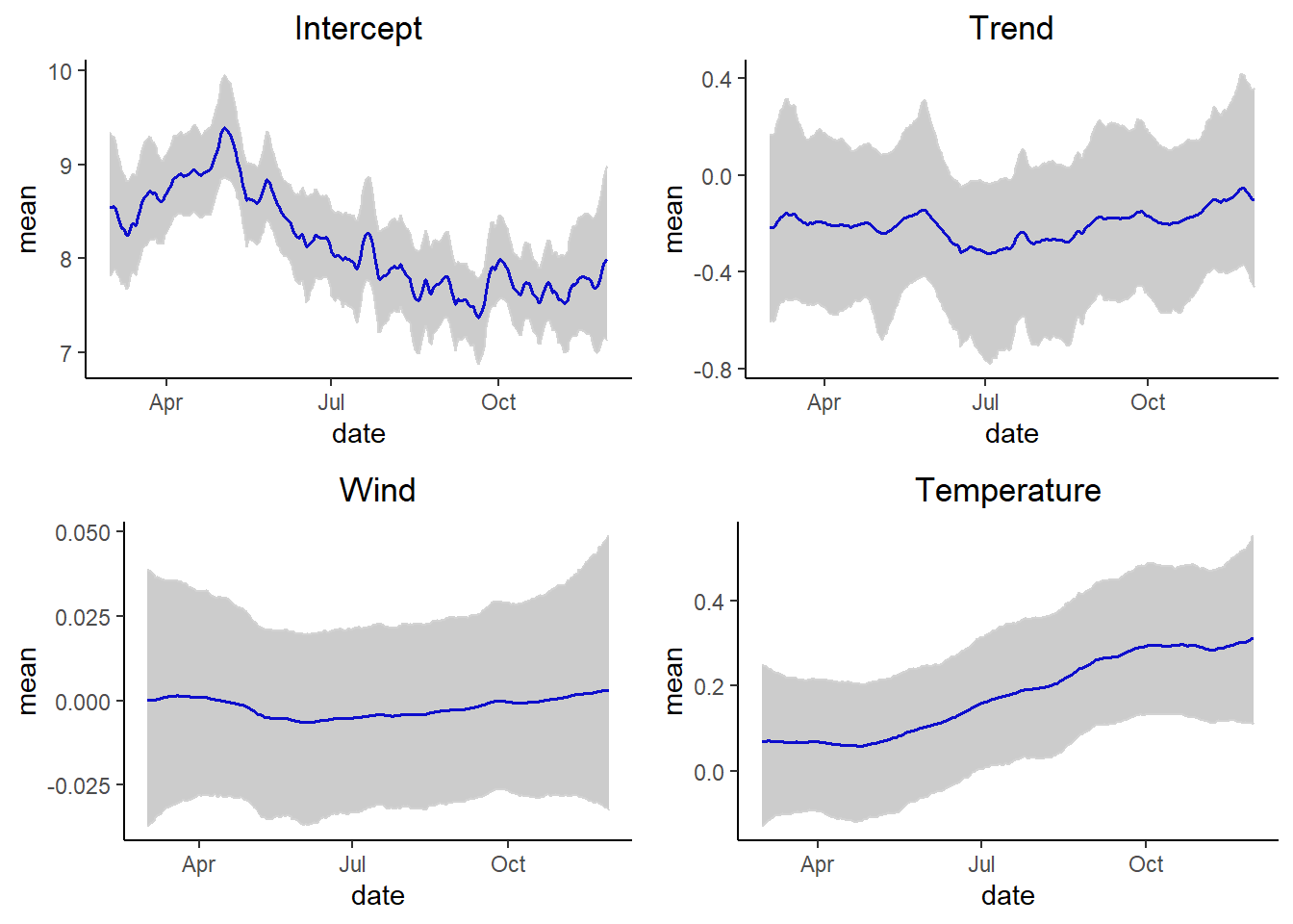
# Fitted values
yfit_summary_dt <- data.frame(yfit_summary) |>
  rownames_to_column() |>
  mutate(time = as.numeric(gsub(".*?([0-9]+).*", "\\1", rowname)))

ggplot(yfit_summary_dt, aes(x = time)) +
  geom_ribbon(aes(ymin = X2.5., ymax = X97.5.),
              alpha = 0.25,
              col = "gray99") +
  geom_point(aes(y = y)) +
  geom_path(aes(y = mean), linewidth = 0.1, size = 1) +
 ylab("Ozone Level (ppm)") +
  xlab("Time") + ggtitle("Fitted values Ozone level UK") +
  theme_classic()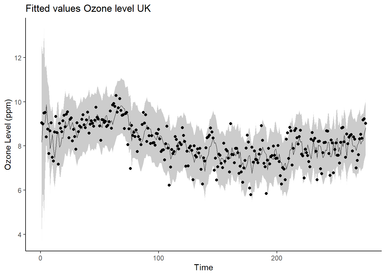
11.1 Example 11.18 Dynamic GLMs for daily counts of carbon monoxide on counts of infant deaths in São Paulo, Brazil
This dataset was analyzed by Alves et al. (2010) and is related to daily counts of deaths of infants under 5 years old due to respiratory causes in São Paulo, Brazil. The sampling period is from January 1, 1994, until 31 December 1997. We fit a simplified version of the model fitted in Alves et al. (2010),
Exercise 11.11
The joint distribution of \(\mathbf{\gamma} = \{\gamma_1, \gamma_2, \dots, \gamma_{N_T}\}\) can be written as: \[ p(\mathbf{\gamma}) = p(\gamma_1) \prod_{t=1}^{N_T-1}p(\gamma_{t+1}\mid\gamma)\\ = p(\gamma_1)(2\pi\sigma_w^2)^{-(N_T-1)/2}\exp\{- \frac{1}{2\sigma_w^2} \sum_{t=1}^{N_T-1} (\gamma_{t+1} - \gamma)^2) \}\\ \propto p(\gamma_1) \exp\{-\frac{1}{2\sigma_w^2}\mathbf{\gamma}^\top M \mathbf{\gamma}\}, \] where the entries of \(M\) are: \[ M_{ij} = \begin{cases} 1, & i = j = 1, N_T\\ 2, & i = j = 2, 3, \dots, N_T - 1 \\ -1 & i = (j-1), \text{where } j = 2, 3, \dots, N_T\\ -1 & i = (j+1), \text{where } j = 1, 2, \dots, N_T - 1 \\ 0 & \text{else} \end{cases}. \] Now, if we assume that \(p(\gamma_1) \propto 1\), i.e., an uninformative, improper prior, we have that \[ p(\mathbf{\gamma}) \propto \exp\{-\frac{1}{2\sigma_w^2}\mathbf{\gamma}^\top M \mathbf{\gamma}\}, \] which implies that, for any \(t\), by Bayes rule,
\[ p(\gamma_t|\mathbf{\gamma}_{-t}) = \frac{p(\mathbf{\gamma})}{p(\mathbf{\gamma}_{-t})} \propto p(\mathbf{\gamma}). \]
Eliminating terms in the joint distribution \(P(\gamma)\) not related to \(\gamma_t\), we obtain
\[ p(\gamma_t|\mathbf{\gamma}_{-t}) \propto \begin{cases} \exp\{-\frac{1}{2\sigma_w^2}(\gamma_t^2 - 2\gamma_t\gamma_{t+1})\}, & t = 1\\ \exp\{-\frac{1}{2\sigma_w^2}(2\gamma_t^2 - 2\gamma_t\gamma_{t+1} - 2\gamma_{t-1}\gamma_t)\}, & t = 2, 3, \dots, N_T-1 \\ \exp\{-\frac{1}{2\sigma_w^2}(\gamma_t^2 - 2\gamma_{t-1}\gamma_{t})\}, & t = N_T \end{cases}. \]
The proportional form implies that these are Normal densities. By completing the square, we can obtain
\[ p(\gamma|\gamma_{-t}) \propto \begin{cases} N(\gamma_{t+1}, \sigma_w^2), & t = 1 \\ N(\frac{\gamma_{t-1}+\gamma_{t+1}}{2}, \sigma^2_w/2), & t = 2, 3 \dots, N_T-1 \\ N(\gamma_{t-1}, \sigma_w^2), & t = N_T \end{cases}, \] as required. A necessary assumption for this conclusion was that \(p(\gamma_1) \propto 1\). ## Exercise 11.12 {-}
The joint density of \(\gamma_t\) and \(\tau_w\), given \(\gamma_{t-1}\) is given by \[ p(\gamma_t, \tau_w \mid \gamma_{t-1}) = \frac{\tau_w^{1/2}}{\sqrt{2\pi}}\exp \left(-\frac{\tau(\gamma_t - \gamma_{t-1})^2}{2} \right) \frac{b^a}{\Gamma(a)}\tau_w^{a-1}\exp(-b\tau_w). \] Marginalizing \(\tau_w\) gives \[ p(\gamma_t \mid \gamma_{t-1}) = \int_{0}^{\infty} \frac{\tau_2^{1/2}}{\sqrt{2\pi}}\exp \left(-\frac{\tau(\gamma_t - \gamma_{t-1})^2}{2} \right) \frac{b^a}{\Gamma(a)}\tau_w^{a-1}\exp(-b\tau_w) d\tau_w \\ = \frac{b^2}{\Gamma(a)\sqrt{2\pi}} \int_{0}^\infty \tau_w^{a-0.5} \exp \left(-\tau_w \left[ \frac{(\gamma_t - \gamma_{t-1})^2}{2} + b\right] \right) d\tau_w \\ = \frac{b^a \Gamma(a+0.5)}{\gamma(a)\sqrt{2\pi} ((\gamma_t - \gamma_{t-1})^2/2+b)^{a+0.5}} \int_{0}^\infty \frac{(\gamma_t - \gamma_{t-1})^2/2+b)^{a+0.5}}{\Gamma(a+0.5)} \tau_w^{(a +0.5) - 1} \exp\left( -\tau_w \left[ \frac{(\gamma_t - \gamma_{t-1})^2}{2} + b\right]\right)\\ = \frac{b^a \Gamma(a+0.5)}{\gamma(a)\sqrt{2\pi} ((\gamma_t - \gamma_{t-1})^2/2+b)^{a+0.5}}, \] where the last equality follows because the integrand was the density of a Gamma distribution. Now, by Bayes rule, we have the following expression for the posterior: \[ p(\tau_{w}|\gamma_t, \gamma_{t-1}) = \frac{p(\gamma_t, \tau_w \mid \gamma_{t-1})}{p(\gamma_t \mid \gamma_{t-1}) } = \frac{((\gamma_t - \gamma_{t-1})^2/2+b)^{a+0.5}}{\Gamma(a + 0.5)}\tau^{(a+0.5)-1} \exp \left(-\tau_w \left[\frac{(\gamma_t - \gamma_{t-1})^2}{2} + b \right] \right), \] which is the density function of the \(Ga(a + 0.5, (\gamma_t - \gamma_{t-1})^2/2 + b)\) distribution. The shape parameter of the posterior is the prior shape parameter shifted by \(0.5\), and the rate parameter is the prior rate parameter shifted by the term \((\gamma_t - \gamma_{t-1})^2/2\).
Exercise 11.13
We use the rjags package here, as it most closely resembles WinBUGS, but is compatible with all operating systems.
## Warning: package 'rjags' was built under R version 4.2.3data <- source("data/pm_london/pm10_London.txt")
inits1 <- source("data/pm_london/11_13_model1_inits1.txt")
model_ar <- jags.model(file = "data/pm_london/11_13_model1.txt",
data = data$value,
inits = inits1$value,
n.chains = 3)## Compiling model graph
## Resolving undeclared variables
## Allocating nodes
## Graph information:
## Observed stochastic nodes: 1410
## Unobserved stochastic nodes: 1514
## Total graph size: 2934
##
## Initializing modelupdate(model_ar, 5000) ## burn in
samples_sigmas <- coda.samples(model_ar,
variable.names = c(
"sigma.v",
"sigma.w"
),
n.iter = 2000,
thin = 2)
plot(samples_sigmas)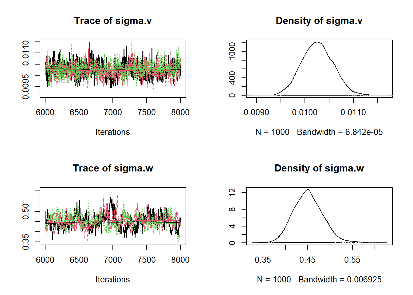
##          sigma.v   sigma.w
## 0%   0.009440187 0.3604371
## 25%  0.010027101 0.4239586
## 50%  0.010254047 0.4472214
## 75%  0.010486342 0.4706450
## 100% 0.011485331 0.6060564
samples_gamma <- coda.samples(model_ar,
variable.names = c(
"gamma",
"y"
),
n.iter = 2000,
thin = 1)
missings <- which(is.na(data$value$y))
nonmissing <- tibble(var = "y", time = as.double(seq(1, length(data$value$y))),
value = data$value$y) |>
filter(!(time %in% missings))
plot_df <- data.frame(samples_gamma[[1]])
plot_df <- plot_df |> pivot_longer(cols = everything(),
names_to = "variable") |>
separate(variable, c("var", "time")) |>
mutate(time = as.numeric(time)) |>
filter(!(var == "y" & !(time %in% missings))) |>
rbind(nonmissing) |>
group_by(var, time) |>
summarise(q025 = quantile(value, prob = 0.025),
q975 = quantile(value, prob = 0.975),
median = median(value))|>
mutate(range = q975-q025)## Warning: Expected 2 pieces. Additional pieces discarded in 5844000 rows [1, 2,
## 3, 4, 5, 6, 7, 8, 9, 10, 11, 12, 13, 14, 15, 16, 17, 18, 19, 20, ...].## `summarise()` has grouped output by 'var'. You
## can override using the `.groups` argument.plot_scatter_df <- plot_df |> dplyr::select(var, time, median) |>
pivot_wider(names_from = var, values_from = median)
plot_scatter <- ggplot(plot_scatter_df, aes(x = y, y = gamma)) +
geom_point(alpha = 0.5)
plot_scatter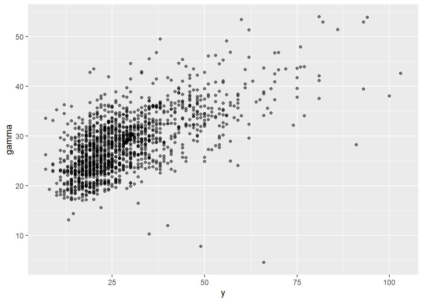
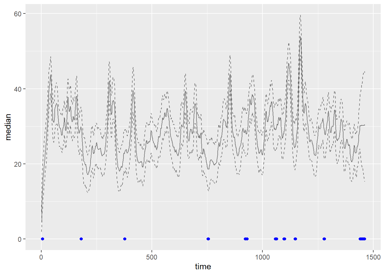
plot <- ggplot(filter(plot_df, var == "gamma"), aes(x = time)) +
  geom_line(aes(y = median), alpha = 0.5) +
  geom_line(aes(y = q025), alpha = 0.5, linetype = "dashed")+
  geom_line(aes(y = q975), alpha = 0.5, linetype = "dashed")+
  geom_point(data = filter(plot_df, (var == "y" & time %in% missings)),
             aes(x = time, y = 0), color = "blue")
plot