Chapter 6 Approaches to Bayesian Computation
This chapter describes methods for implementing Bayesian models when their complexity means that simple, analytic solutions may not be available. The reader will have gained an understanding of the following topics:
analytical approximations to the posterior distribution;
use of samples from a posterior distribution for inference and Monte Carlo integration;
methods for direct sampling such as importance and rejection sampling;
Markov Chain Monte Carlo (MCMC) and methods for obtaining samples from the required posterior distribution including Metropolis–Hastings and Gibbs algorithms;
use of NIMBLE and RStan packages to fit Bayesian models using Gibbs sampling;
Integrated Nested Laplace Approximations (INLA) as a method for performing efficient Bayesian inference including the use of R-INLA to implement a wide variety of latent Gaussian models.
Example 6.2: Gibbs sampling with a Poisson-Gamma model - hospital admissions for chronic obstructive pulmonary disease (COPD) for England between 2001-2010
We now look at example into the hospital admission rates for chronic obstructive pulmonary disease (COPD) in England between 2001–2010.
In England, there are 324 local authority administrative areas each with an observed and expected number of cases. The expected numbers were calculated using indirect standardization by applying the age–sex specific rates for the whole of England to the age–sex population profile of each of the areas.
We show the full conditional distributions for a Poisson model where the prior distribution on the rates is Gamma, that is, \(y_i \mid \theta_, E_i \sim Poi(\theta_i E_i)\) where \(E_i\) is the expected number of cases in area \(i\). In particular, let \(\mathbf{y} = (y_1, ..., y_N)\) be a \(N\)-dimensional vector with observed counts on the total number of hospital admissions for chronic obstructive pulmonary disease (COPD) for England between 2001 and 2010. The expected numbers of hospital admissions by local authority were computed as described in Chapter 2, Section 2.1.
If we assign a Gamma prior to the random effects \(\theta_i\), i.e., \(\theta_i \sim Gamma(a, b)\) for \(i=1, \dots N\), and independent exponential distributions to the hyperparameters \(a\) and \(b\) then we can find the full conditional distributions required for Gibbs sampling.
The joint posterior is proportional to
\[\begin{eqnarray} \nonumber p(a, b, \mathbf{\theta} | \mathbf{y}) &\propto& \prod^N _{i=1} \frac{\left(\theta_i E_i\right)^{y_i}}{y_i!} \exp(-\theta_i E_i) \, \frac{b^{a}}{\Gamma (a) }\theta_i^{a-1} e^{-b \theta_i} \\ \nonumber && \times \lambda_{a} \exp(-\lambda_{a}) \, \lambda_{b}\exp(-\lambda_{b}), \end{eqnarray}\] and the full conditionals are:
- Posterior full conditional for each \(\theta_i\), \(i=1,\dots,N\): \[\begin{eqnarray} p(\theta_i | \mathbf{\theta}_{-i}, a, b, \mathbf{y}) \propto \theta_i^{y_i+a-1} \exp[-(E_i+b)\theta_i], \end{eqnarray}\] which is the kernel of a Gamma distribution with parameters \(y_i+a\) and \(E_i+b\);
- Posterior full conditional for \(b\): \[\begin{eqnarray} p(b | \mathbf{\theta}, a, \mathbf{y}) \propto b^{N a} \exp\left[-\left(\sum^N_{i=1}\theta_i + \lambda_{b}\right)b\right], \end{eqnarray}\] which is the kernel of a Gamma distribution with parameters \(Na+1\) and \((\sum^N_{i=1}\theta_i + \lambda_{b})\);
- Posterior full conditional for \(a\): \[\begin{eqnarray} p(a | \mathbf{\theta}, b, \mathbf{y}) \propto \frac{\left(b^N \prod^N_{i=1}\theta_i\right)^{a-1}}{\Gamma (a)^N }, \end{eqnarray}\] which does not have a closed form. We propose to sample from \(p(a | \mathbf{\theta}, b, \mathbf{y})\) through a random walk, Metropolis-Hastings step. As \(a\) must be strictly positive, the proposal is a log-normal distribution whose associated normal distribution has mean at the logarithm of the current value and some fixed variance, say \(u\), that needs to be tuned.
For this example, the following packages are needed ggplot2 and sf.
Load the necessary packages.
To create SMR maps, we need to load the relevant shapefiles into the R session.
- englandlocalauthority.shp and englandlocalauthority.dbf contain the location, shape, and attributes of English local authorities. The function
read_sf()from thesfpackage will read these shapefiles intoR. - copdmortalityobserved.csv contains the observed number of hospital admissions in England by local authority. You can find this data by clicking.
- copdmortalityexpected.csv contains the expected number of hospital admissions in England by local authority.
# Reading in the borders of the shape file
england <- read_sf("data/copd/englandlocalauthority.shp")
# Reading the data
observed <-read.csv(file = "data/copd/copdmortalityobserved.csv", row.names = 1)
expected <-read.csv(file = "data/copd/copdmortalityexpected.csv", row.names = 1)
Print summaries of the observed and expected counts.
##                         name Y2001 Y2002 Y2003 Y2004 Y2005 Y2006 Y2007 Y2008
## 00AA      City of London LB      2     0     3     1     1     1     5     1
## 00AB Barking and Dagenham LB   100   100   122    93   136    97    91    96
## 00AC               Barnet LB   110   102   106    89    99    97    72    84
## 00AD               Bexley LB   109   113   113    96   113    97    94    89
## 00AE                Brent LB    69    89    70    59    61    48    53    46
## 00AF              Bromley LB   120   129   135   124   128   117   120   106
##      Y2009 Y2010
## 00AA     0     1
## 00AB   101    78
## 00AC    78    89
## 00AD    93    93
## 00AE    55    43
## 00AF 107 113## E2001 E2002 E2003 E2004 E2005 E2006
## 00AA 2.648915 2.68106 2.727112 2.749562 2.808655 2.915977
## 00AB 63.946730 63.41700 62.567863 61.444884 60.677119 59.678672
## 00AC 121.795213 121.91534 122.451050 123.201898 124.449563 125.982868
## 00AD 90.201336 91.24645 91.949050 92.754781 93.674540 94.598593
## 00AE 76.876437 77.18529 78.017980 78.967493 80.422828 81.785325
## 00AF 131.182934 132.30521 133.257442 134.520920 136.441229 137.382528
## E2007 E2008 E2009 E2010
## 00AA 3.021586 3.114696 3.237998 3.237998
## 00AB 58.487583 57.701932 57.250524 57.250524
## 00AC 127.088805 128.825149 131.374946 131.374946
## 00AD 95.447131 96.832061 97.651369 97.651369
## 00AE 83.651266 85.265264 87.089119 87.089119
## 00AF 138.634021 139.508507 140.634084 140.634084## name Y2001 Y2002 Y2003
## Length:324 Min. : 2.00 Min. : 0.00 Min. : 3.00
## Class :character 1st Qu.: 35.00 1st Qu.: 38.00 1st Qu.: 38.00
## Mode :character Median : 50.00 Median : 52.00 Median : 52.00
## Mean : 68.01 Mean : 69.63 Mean : 73.44
## 3rd Qu.: 83.50 3rd Qu.: 80.75 3rd Qu.: 83.25
## Max. :445.00 Max. :438.00 Max. :480.00
## Y2004 Y2005 Y2006 Y2007
## Min. : 1.00 Min. : 1.00 Min. : 1.00 Min. : 5.00
## 1st Qu.: 35.00 1st Qu.: 37.00 1st Qu.: 35.00 1st Qu.: 37.00
## Median : 49.50 Median : 51.00 Median : 49.00 Median : 50.00
## Mean : 66.67 Mean : 69.37 Mean : 67.07 Mean : 68.17
## 3rd Qu.: 81.25 3rd Qu.: 80.50 3rd Qu.: 81.00 3rd Qu.: 79.00
## Max. :428.00 Max. :395.00 Max. :428.00 Max. :456.00
## Y2008 Y2009 Y2010
## Min. : 1.00 Min. : 0.00 Min. : 1.00
## 1st Qu.: 37.00 1st Qu.: 36.00 1st Qu.: 38.00
## Median : 51.00 Median : 50.00 Median : 51.00
## Mean : 71.40 Mean : 67.04 Mean : 68.81
## 3rd Qu.: 84.25 3rd Qu.: 78.00 3rd Qu.: 81.25
## Max. :463.00 Max. :394.00 Max. :441.00## E2001 E2002 E2003 E2004
## Min. : 2.649 Min. : 2.681 Min. : 2.727 Min. : 2.75
## 1st Qu.: 39.066 1st Qu.: 39.456 1st Qu.: 39.849 1st Qu.: 40.60
## Median : 51.766 Median : 52.671 Median : 53.487 Median : 54.29
## Mean : 62.944 Mean : 63.589 Mean : 64.139 Mean : 64.72
## 3rd Qu.: 74.292 3rd Qu.: 74.974 3rd Qu.: 74.701 3rd Qu.: 74.02
## Max. :370.913 Max. :371.271 Max. :369.861 Max. :368.87
## E2005 E2006 E2007 E2008
## Min. : 2.809 Min. : 2.916 Min. : 3.022 Min. : 3.115
## 1st Qu.: 41.646 1st Qu.: 42.497 1st Qu.: 43.203 1st Qu.: 44.262
## Median : 54.765 Median : 55.506 Median : 56.552 Median : 57.522
## Mean : 65.440 Mean : 66.180 Mean : 67.022 Mean : 67.950
## 3rd Qu.: 75.003 3rd Qu.: 75.260 3rd Qu.: 75.790 3rd Qu.: 76.935
## Max. :368.565 Max. :367.838 Max. :368.026 Max. :368.291
## E2009 E2010
## Min. : 3.238 Min. : 3.238
## 1st Qu.: 45.062 1st Qu.: 45.062
## Median : 58.077 Median : 58.077
## Mean : 68.901 Mean : 68.901
## 3rd Qu.: 78.166 3rd Qu.: 78.166
## Max. :368.940 Max. :368.940Modelling the raw standardized mortality rates (SMRs)
Calculate the raw SMRs as
\[ \text{SMR} = \frac{observed}{expected}\]
SMR_raw <- observed[, -1] / expected

# Rename columns
names(SMR_raw) <-
  c("SMR2001",
    "SMR2002",
    "SMR2003",
    "SMR2004",
    "SMR2005",
    "SMR2006",
    "SMR2007",
    "SMR2008",
    "SMR2009",
    "SMR2010"
  )
# Printing first six rows of raw SMRs
head(SMR_raw)
## SMR2001 SMR2002 SMR2003 SMR2004 SMR2005 SMR2006 SMR2007
## 00AA 0.7550261 0.0000000 1.1000648 0.3636943 0.3560423 0.3429382 1.6547601
## 00AB 1.5638016 1.5768644 1.9498828 1.5135516 2.2413721 1.6253713 1.5558858
## 00AC 0.9031554 0.8366462 0.8656520 0.7223915 0.7955030 0.7699460 0.5665330
## 00AD 1.2084078 1.2384043 1.2289415 1.0349871 1.2063043 1.0253852 0.9848384
## 00AE 0.8975442 1.1530694 0.8972291 0.7471429 0.7584911 0.5869024 0.6335828
## 00AF 0.9147531 0.9750183 1.0130766 0.9217897 0.9381329 0.8516367 0.8655884
## SMR2008 SMR2009 SMR2010
## 00AA 0.3210586 0.0000000 0.3088328
## 00AB 1.6637225 1.7641760 1.3624329
## 00AC 0.6520466 0.5937205 0.6774503
## 00AD 0.9191171 0.9523676 0.9523676
## 00AE 0.5394928 0.6315370 0.4937471
## 00AF 0.7598103 0.7608397 0.8035037## SMR2001 SMR2002 SMR2003 SMR2004
## Min. :0.3883 Min. :0.0000 Min. :0.3616 Min. :0.2778
## 1st Qu.:0.7900 1st Qu.:0.8272 1st Qu.:0.8519 1st Qu.:0.7636
## Median :0.9496 Median :1.0168 Median :1.0209 Median :0.9266
## Mean :1.0349 Mean :1.0508 Mean :1.0895 Mean :0.9812
## 3rd Qu.:1.2526 3rd Qu.:1.2364 3rd Qu.:1.3071 3rd Qu.:1.1858
## Max. :1.9861 Max. :2.2181 Max. :2.2483 Max. :1.9811
## SMR2005 SMR2006 SMR2007 SMR2008
## Min. :0.3326 Min. :0.3429 Min. :0.3509 Min. :0.3211
## 1st Qu.:0.7592 1st Qu.:0.7415 1st Qu.:0.7533 1st Qu.:0.7695
## Median :0.9573 Median :0.9101 Median :0.9305 Median :0.9404
## Mean :1.0126 Mean :0.9726 Mean :0.9743 Mean :1.0069
## 3rd Qu.:1.2083 3rd Qu.:1.1586 3rd Qu.:1.1679 3rd Qu.:1.1979
## Max. :2.2414 Max. :2.0805 Max. :1.8528 Max. :2.0567
## SMR2009 SMR2010
## Min. :0.0000 Min. :0.3088
## 1st Qu.:0.7452 1st Qu.:0.7682
## Median :0.8777 Median :0.9337
## Mean :0.9328 Mean :0.9639
## 3rd Qu.:1.0934 3rd Qu.:1.1335
## Max. :1.8507 Max. :2.3856Attach the values of the raw SMRs to the shapefiles. The function merge() allows us to combine a data frame with a shapefile to plot later.
# Convert row names to ID column
SMR_raw <- tibble::rownames_to_column(SMR_raw, "ID")
# Combine raw SMRs and shapefiles
SMRspatial_raw <- merge(england, SMR_raw, by = "ID")
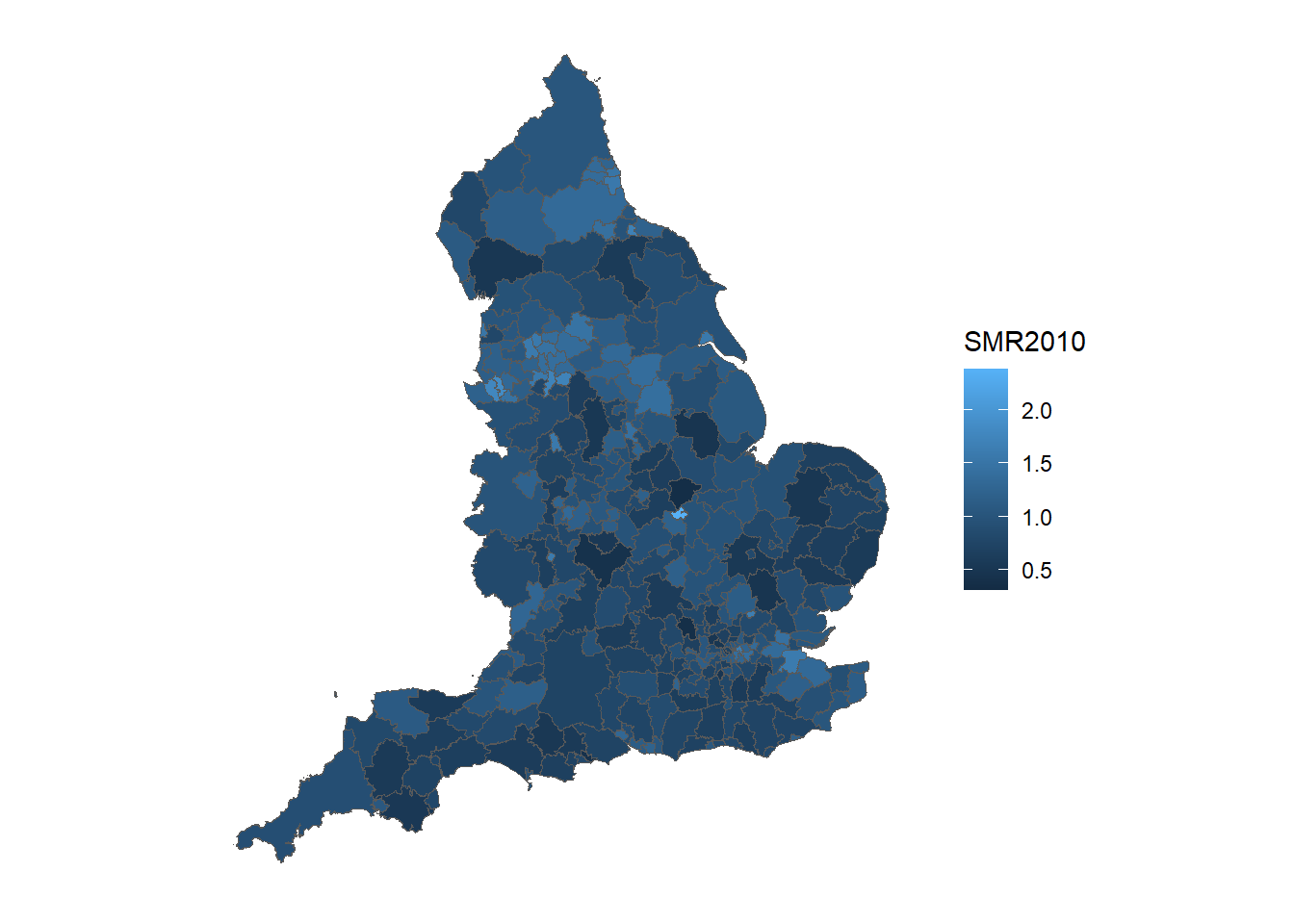
Use ggplot() and geom_sf() to create a choropleth map such that local authorities are colored by the raw SMR estimate.
# Creating breaks for legend in plot
range <-seq(min(SMR_raw$SMR2010) - 0.01,
      max(SMR_raw$SMR2010) + 0.01,
      length.out = 11)

# Creating the map of Raw SMRs in England in 2010
ggplot() +
  # Choose spatial object and column for plotting
  geom_sf(data = SMRspatial_raw, aes(fill = SMR2010)) +
  # Break points for colours
  scale_y_continuous(breaks = range) +
  # Clear background and plot borders
  theme(
    axis.text.x = element_blank(),
    axis.text.y = element_blank(),
    axis.ticks = element_blank(),
    rect = element_blank()
) 
MCMC implementation of the Poisson-Gamma model in R
The following code shows how to implement the MCMC using R for the COPD example.
We start by defining the constants and the vectors that will be used in the code.
# observations
y <- observed$Y2010
# offset
E <- expected$E2010
# Number of MCMC iterations
L <- 20000

## Initialize objects used in MCMC
# Matrix for sampled values of parameter theta_i
theta <-matrix(ncol = length(y), nrow = L)
# Matrix for fitted values
fitted <-theta
# Vector for sampled values of hyper-parameter a
a <- c()
# Vector for sampled values of hyper-parameter b
b <- c()

## Define constants
# Sample size
N <- length(y)
# Parameter of exponential prior for a
lambda_a <- 1
# Parameter of exponential prior for b
lambda_b <- 1
# standard deviation of the proposal distribution of log a
u <- 0.1
# Initialize theta
theta[1, ] <- y / E
# Initial value sampled from the prior for a
# REVIEW: In the example of the book theta ~ Ga(a,a) not Ga(a,b)
a <- rexp(1, lambda_a)
# Initial value sampled from the prior for b
b <- rexp(1, lambda_b)
fitted[1, ] <- rpois(N, E * theta[1, ])


# Once all the constants and initial values are set we can run the MCMC.
# The following code shows the MCMC implementation of a Poisson-Gamma model using only `R`.
# Starting from l=2 as l=1 contains the initial values
for(l in 2:L) {

# Sampling from the posterior full conditional of each theta_i
  for (i in 1:N)
    theta[l, i] <- rgamma(1, (y[i] + a[(l - 1)]), rate = (E[i] + b[(l - 1)]))
  # Sampling from the posterior full conditional of b
  b[l] <- rgamma(1, (N * a[(l - 1)] + 1), rate = (sum(theta[l, ]) + lambda_b))
  # Metropolis-Hastings step to sample from the full conditional of "a"
  # the new value receives the current value in case the proposed
  # value is rejected
  a[l] <- a[l - 1]
  # Proposal in the log-scale
  laprop <- rnorm(1, log(a[l - 1]), u)
  aprop <- exp(laprop)
  #computing the numerator of the M-H step
  num <- N * (aprop * (log(b[l])) - lgamma(aprop)) + (aprop - 1) * sum(log(theta[l, ])) -
    aprop * lambda_a + log(aprop)
  #computing the denominator of the M-H step
  den <- N * (a[l - 1] * (log(b[l])) - lgamma(a[l - 1])) + (a[(l - 1)] - 1) * sum(log(theta[l, ])) -
    a[(l - 1)] * lambda_a + log(a[(l - 1)])
  #computing the M-H ratio
  ratio <- exp(num - den)
  unif <- runif(1)
  # Change the current value if the proposed value is accepted
  if (unif < ratio)
    a[l] <- aprop
  fitted[l,] <- rpois(N, E * theta[l,])
}
After running the MCMC, check convergence of the chains using trace plots, autocorrelation functions and functions from the coda package.
# Number of burn in samples and thinning
burnin <- 10000
thin <- 10

# MCMC samples, setting the burnin and thinning
seqaux <- seq(burnin, L, by = thin)

# Trace-plots of the parameters
xx <- seq(0, 20, length = 3000)

par(mfrow = c(3, 2),pty="m")
# Plot for "a"
#traceplot for the posterior sample of parameters 'a' and 'b'
plot(a[seqaux], type = "l", bty = "n",xlab="Iterations",ylab="a")
plot(b[seqaux], type = "l", bty = "n",xlab="Iterations",ylab="b")
#histogram of the posterior distribution of parameter 'a'
hist(a[seqaux], prob = 1, main = "",)
#prior distribution of parameter "a'
lines(xx, dexp(xx, lambda_a), col = 2, lwd = 2)
hist(b[seqaux], prob = 1, main = "")
#prior distribution of parameter "a'
lines(xx, dexp(xx, lambda_b), col = 2, lwd = 2)
#autocorrelation function of the sampled values of parameter 'a'
acf(a[seqaux],main="ACF for a")
acf(b[seqaux],main="ACF for b")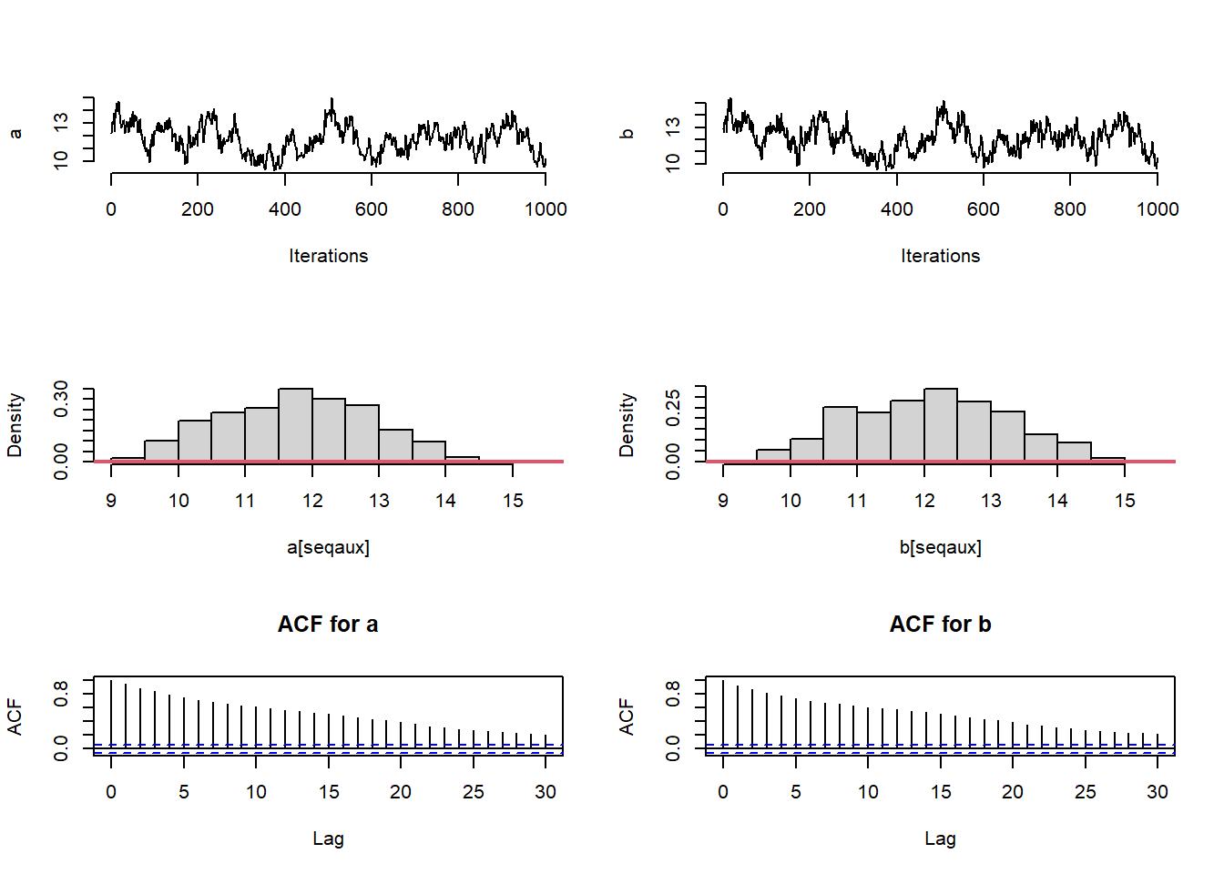
# Traceplots of the posterior samples of some of the theta's
par(mfrow = c(3, 3))
for (i in 1:9)
  plot(theta[seqaux, i], type = "l", bty = "n",xlab='Iteration',ylab=expression(paste(theta,i)))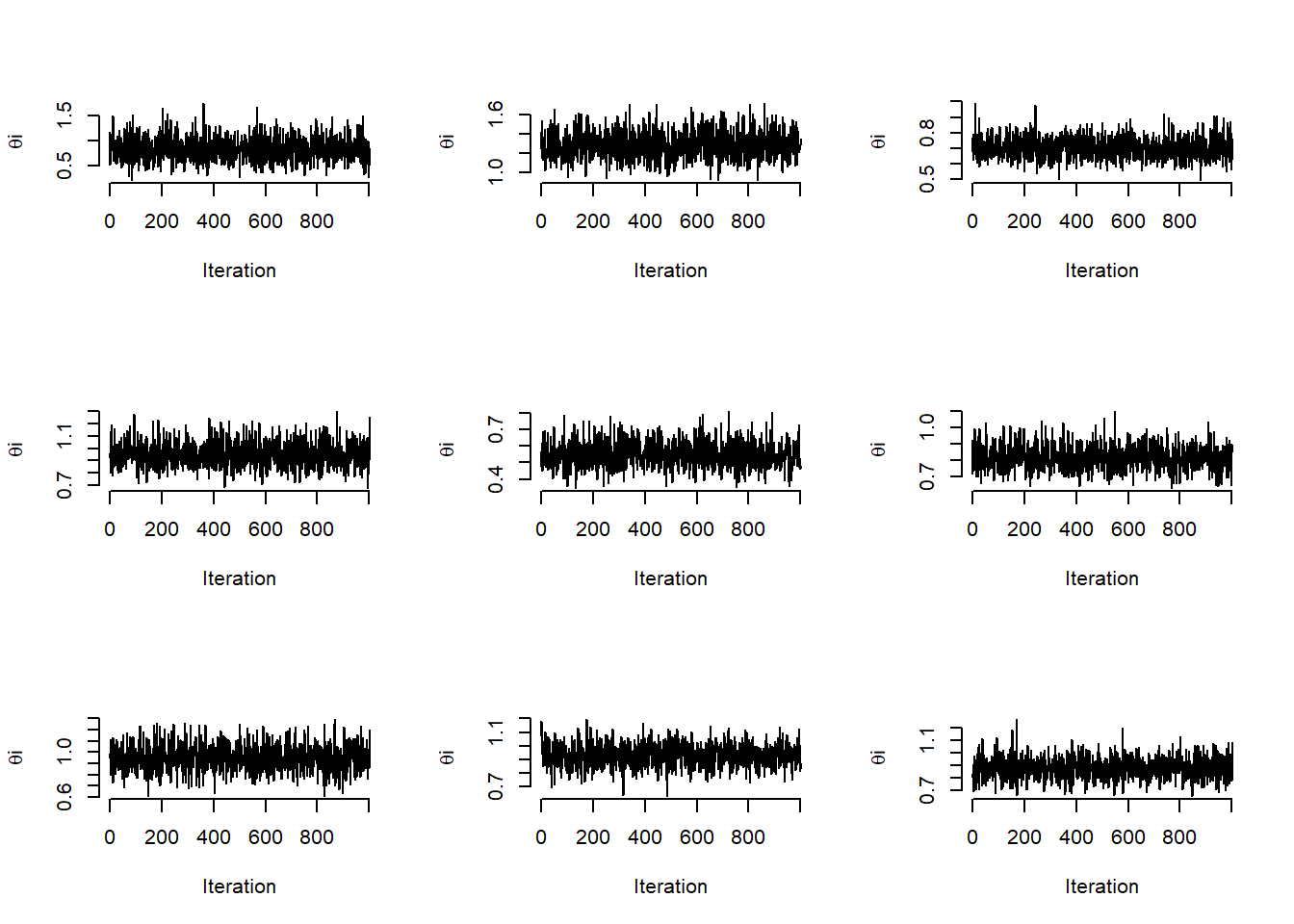
Other diagnostic tools that can be assessed are the effective sample size (ESS) and Rhat. This can be done using the package coda.
## [1] "ESS a: 32.126114421714"## [1] "ESS b: 30.2610882715984"## [1] "ESS theta[1]: 1001"## [1] "ESS theta[10]: 1001"From the trace-plots and the ESS of the sampled values for parameters a and b it looks like the sampled values are highly auto-correlated. We can run the MCMC longer to get a bigger or ESS, or we can tune the variance of the proposal of a to decrease the auto-correlation among sampled values. To this end, we use the algorithm proposed by Roberts and Rosenthal (2001)
# observations
y <- observed$Y2010
# offset
E <- expected$E2010
# Number of MCMC iterations
L <- 30000
burnin<-10000
check<-50
attempt<-0
accept<-0

## Initialize objects used in MCMC
# Matrix for sampled values of parameter theta_i
theta <-matrix(ncol = length(y), nrow = L)
# Matrix for fitted values
fitted <-theta
# Vector for sampled values of hyper-parameter a
a <- c()
# Vector for sampled values of hyper-parameter b
b <- c()

## Define constants
# Sample size
N <- length(y)
# Parameter of exponential prior for a
lambda_a <- 1
# Parameter of exponential prior for b
lambda_b <- 1
# standard deviation of the proposal distribution of log a
u <- 0.1
# Initialize theta
theta[1, ] <- y / E
# Initial value sampled from the prior for a
# REVIEW: In the example of the book theta ~ Ga(a,a) not Ga(a,b)
a <- rexp(1, lambda_a)
# Initial value sampled from the prior for b
b <- rexp(1, lambda_b)
fitted[1, ] <- rpois(N, E * theta[1, ])
k<-0

# Once all the constants and initial values are set we can run the MCMC.
# The following code shows the MCMC implementation of a Poisson-Gamma model using only `R`.
# Starting from l=2 as l=1 contains the initial values
for(l in 2:L) {

# Sampling from the posterior full conditional of each theta_i
  for (i in 1:N)
    theta[l, i] <- rgamma(1, shape=(y[i] + a[(l - 1)]), rate =(E[i] + b[(l - 1)]))
  # Sampling from the posterior full conditional of b
  b[l] <- rgamma(1, shape=(N * a[(l - 1)] + 1), rate=(sum(theta[l, ]) + lambda_b))
  # Metropolis-Hastings step to sample from the full conditional of "a"
  # the new value receives the current value in case the proposed
  # value is rejected
  a[l] <- a[l - 1]
  # Proposal in the log-scale
  laprop <- rnorm(1, log(a[l - 1]), u)
  aprop <- exp(laprop)
  #computing the numerator of the M-H step
  num <- N * ((aprop) * (log(b[l])) - lgamma(aprop)) + (aprop - 1) * sum(log(theta[l, ])) -
    aprop * lambda_a + log(aprop)
  #computing the denominator of the M-H step
  den <- N * ((a[l - 1]) * (log(b[l])) - lgamma(a[l - 1])) +
    (a[(l - 1)] - 1) * sum(log(theta[l, ])) - a[(l - 1)] * lambda_a + log(a[(l - 1)])
  #computing the M-H ratio
  attempt<-attempt+1
  ratio <- exp(num - den)
  unif <- runif(1)
  # Change the current value if the proposed value is accepted
  if (unif < ratio){
    accept<-accept+1
    a[l] <- aprop
  }
  # TUNING!
  if(l<burnin & attempt==check){
    K<-k+1
    print(paste0("Can sd of ", round(u,3),
                   " for a gave acc rate ",accept/attempt))
    delta<-min(0.01,1/sqrt(k+1))
    if(accept/attempt>0.44){u<-u*exp(delta)}
    if(accept/attempt<0.44){u<-u*exp(-delta)}
    accept <- attempt <- 0
   #   if(accept/attempt<0.2){u<-u*0.8}
  #    if(accept/attempt>0.6){u<-u*1.2}
  #    accept <- attempt <- 0
    }
  fitted[l,] <- rpois(N, E * theta[l,])
}
# Number of burn in samples and thinning
burnin <- 10000
thin <- 1
# MCMC samples, setting the burnin and thinning
seqaux <- seq(burnin, L, by = thin)
# Trace-plots of the parameters
xx <- seq(0, 20, length = 3000)
par(mfrow = c(3, 2),pty="m")
# Plot for "a"
#traceplot for the posterior sample of parameters 'a' and 'b'
plot(a[seqaux], type = "l", bty = "n",xlab="Iterations",ylab="a")
plot(b[seqaux], type = "l", bty = "n",xlab="Iterations",ylab="b")
#histogram of the posterior distribution of parameter 'a'
hist(a[seqaux], prob = 1, main = "",)
#prior distribution of parameter "a'
lines(xx, dexp(xx, lambda_a), col = 2, lwd = 2)
hist(b[seqaux], prob = 1, main = "")
#autocorrelation function of the sampled values of parameter 'a'
acf(a[seqaux],main="ACF for a")
acf(b[seqaux],main="ACF for b")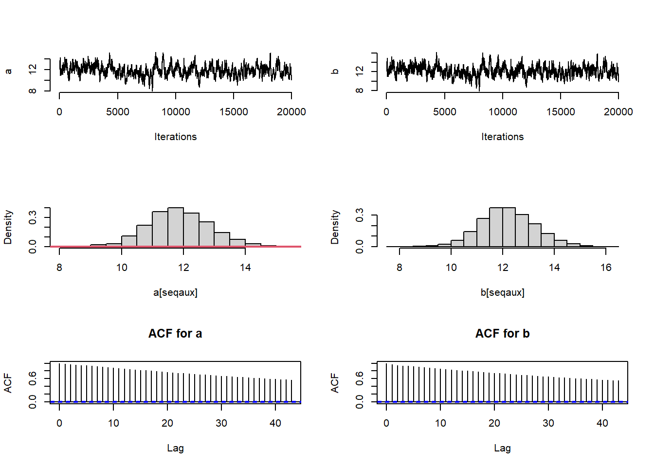
## [1] "ESS a: 123.907829891743"## [1] "ESS b: 134.452182190428"## [1] "ESS theta[1]: 19286.3773745989"## [1] "ESS theta[10]: 20001.0000000001"The ESS of a and b have increased a bit. Another way to increase the ESS is to run the algorithm for multiple chains starting from different values.
# Posterior summaries of theta_i
meantheta <- apply(theta, 2, mean)
q025theta <- apply(theta, 2, function(x)
  quantile(x, 0.025))
q975theta <- apply(theta, 2, function(x)
  quantile(x, 0.975))

# Plot the mean and 95% CIs for the thetas

par(mfrow = c(1, 1))
plot(
  meantheta,
  pch = 19,
  cex = 0.8,
  bty = "n",
  xlab = "Borough",
  ylab = "Posterior Summary Rate",
  ylim = c(min(q025theta), max(q975theta))
)
for (i in 1:N)
  segments(i, q025theta[i], i, q975theta[i])
abline(h = 1, lwd = 2, lty = 2)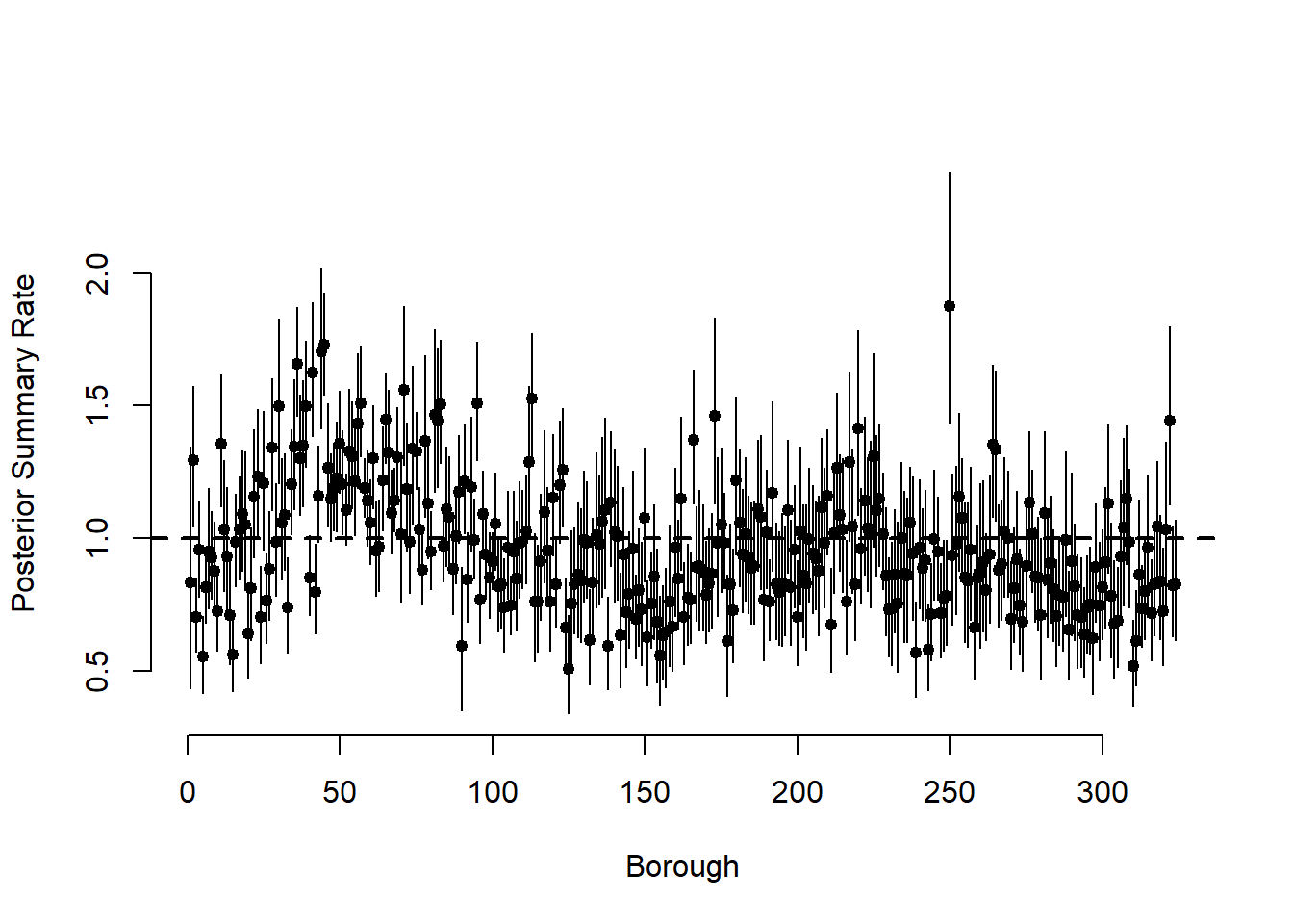
# Posterior summary of fitted values

meanfit <- apply(fitted, 2, mean)
q025fit <- apply(fitted, 2, function(x)
  quantile(x, 0.025))
q975fit <- apply(fitted, 2, function(x)
  quantile(x, 0.975))

# Plot mean and 95% CIs for the fitted values

par(mfrow = c(1, 1))
plot(
  y,
  meanfit,
  ylim = c(min(q025fit), max(q975fit)),
  xlab = "Observed",
  ylab = "Fitted",
  pch = 19,
  cex = 0.7,
  bty = "n"
)
for (i in 1:N)
  segments(y[i], q025fit[i], y[i], q975fit[i])
abline(a = 0, b = 1)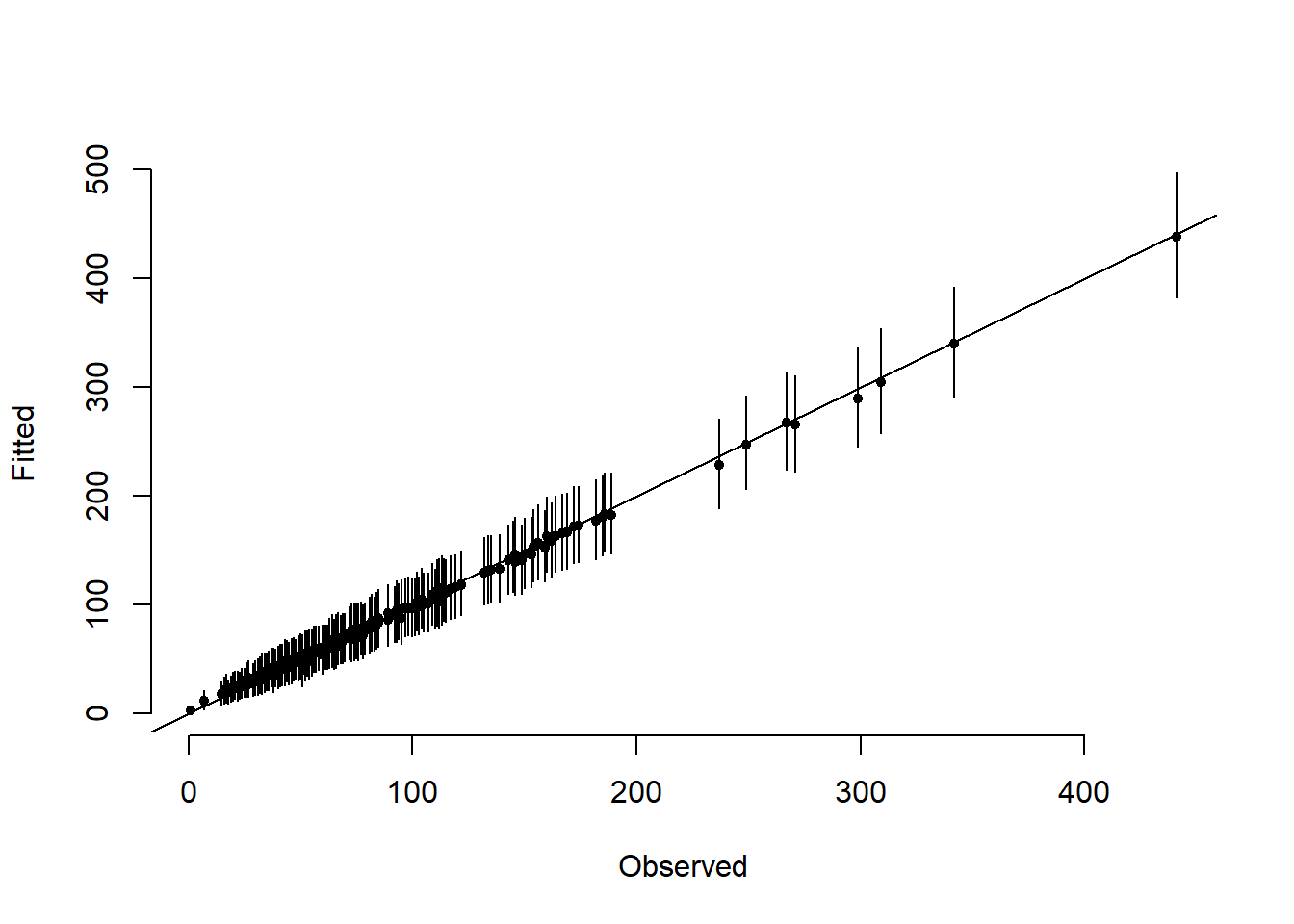
We now show how to run the same model using Nimble.
Code for the Poisson-Gamma model in Nimble
require("nimble")
# Define the model
Example6_2Code <- nimbleCode({
  for (i in 1:N) {
    Y[i] ~ dpois(mu[i])
    mu[i] <- log(E[i]) * theta[i]
    theta[i] ~ dgamma(a,b)
  }

  # Priors
  a ~ dexp(1)
  b ~ dexp(1)

})

# Read the data and define the constants, data and initials lists for the `Nimble` model.

ex.const <- list(
  E = expected$E2010,
  N=length(observed$Y2010))

ex.data <- list(Y = observed$Y2010)

inits <- function()
  list(theta = rgamma(length(y),1,1),a=rexp(1,1),b=rexp(1,1))

# Define parameters to monitor and run the model

params <- c("a", "b", "theta")

mcmc.out <- nimbleMCMC(
  code = Example6_2Code,
  data = ex.data,
  constants = ex.const,
  inits = inits,
  monitors = params,
  niter = 22000,
  nburnin = 2000,
  thin = 10,
  WAIC = TRUE,
  nchains = 2,
  samplesAsCodaMCMC = TRUE
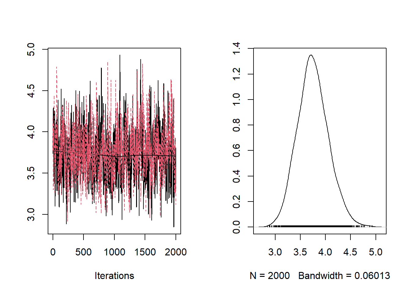
)
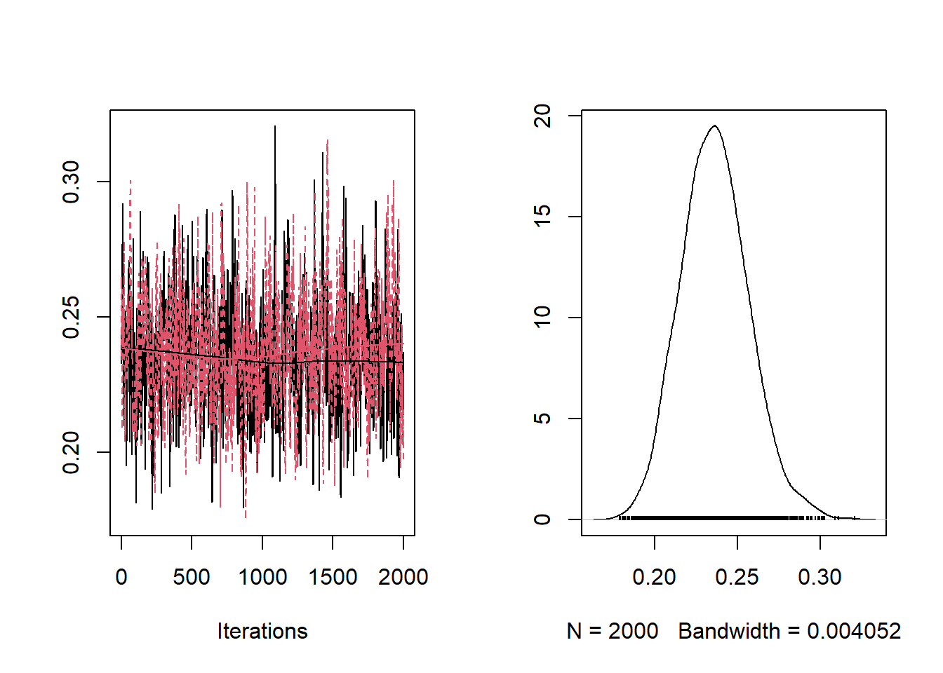
Example 6.3: Fitting a Poisson regression model
In this example, we consider the Poisson log-linear model seen in Chapter 2, Section 2.7. We consider the observed and expected number of cases of respiratory mortality in small areas in the UK from a study examining the long-term effects of air pollution (Elliott, Shaddick, Wakefield, de Hoogh, & Briggs, 2007).
\[\begin{eqnarray} \label{eqn:cum1c2} \log \mu_{l} = \beta_0 + \beta_1 X_{l} + \beta_{d}X_{l} \end{eqnarray}\] where \(\beta_1\) represents the effect of exposure and \(\beta_d\) is the effect of the area-level covariate.
Nimble
Load nimble package
The NIMBLE code to fit this model is as follows:
# Define the model
Example6_3Code <- nimbleCode({
  for (i in 1:N) {
    Y[i] ~ dpois(mu[i])
    log(mu[i]) <- log(E[i]) + beta0 + beta1 * X1[i] + beta2 * X2[i]
  }

  # Priors
  beta0 ~ dnorm (0 , sd = 100)
  beta1 ~ dnorm (0 , sd = 100)
  beta2 ~ dnorm (0 , sd = 100)

  # Functions of interest:
  base <- exp(beta0)
  RR <- exp(beta1)
})

# Read the data and define the constants, data and initials lists for the `Nimble` model.

# REVIEW: Is this another version of the COPD data? Is there a data dictionary for this dataset?

data <- read.csv("data/DataExample53.csv", sep = ",")

ex.const <- list(
  N = nrow(data),
  E = data$exp_lungc65pls,
  X1 = as.vector(scale(data$k3)),
  X2 = as.vector(scale(data$k2))
)

ex.data <- list(Y = data$lungc65pls)

inits <- function()
  list(beta0 = rnorm(1),
       beta1 = rnorm(1),
       beta2 = rnorm(1))

# Define parameters to monitor and run the model

params <- c("beta0", "beta1", "beta2", "base", "RR")

mcmc.out <- nimbleMCMC(
  code = Example6_3Code,
  data = ex.data,
  constants = ex.const,
  inits = inits,
  monitors = params,
  niter = 22000,
  nburnin = 2000,
  thin = 10,
  WAIC = TRUE,
  nchains = 3,
  samplesAsCodaMCMC = TRUE
)
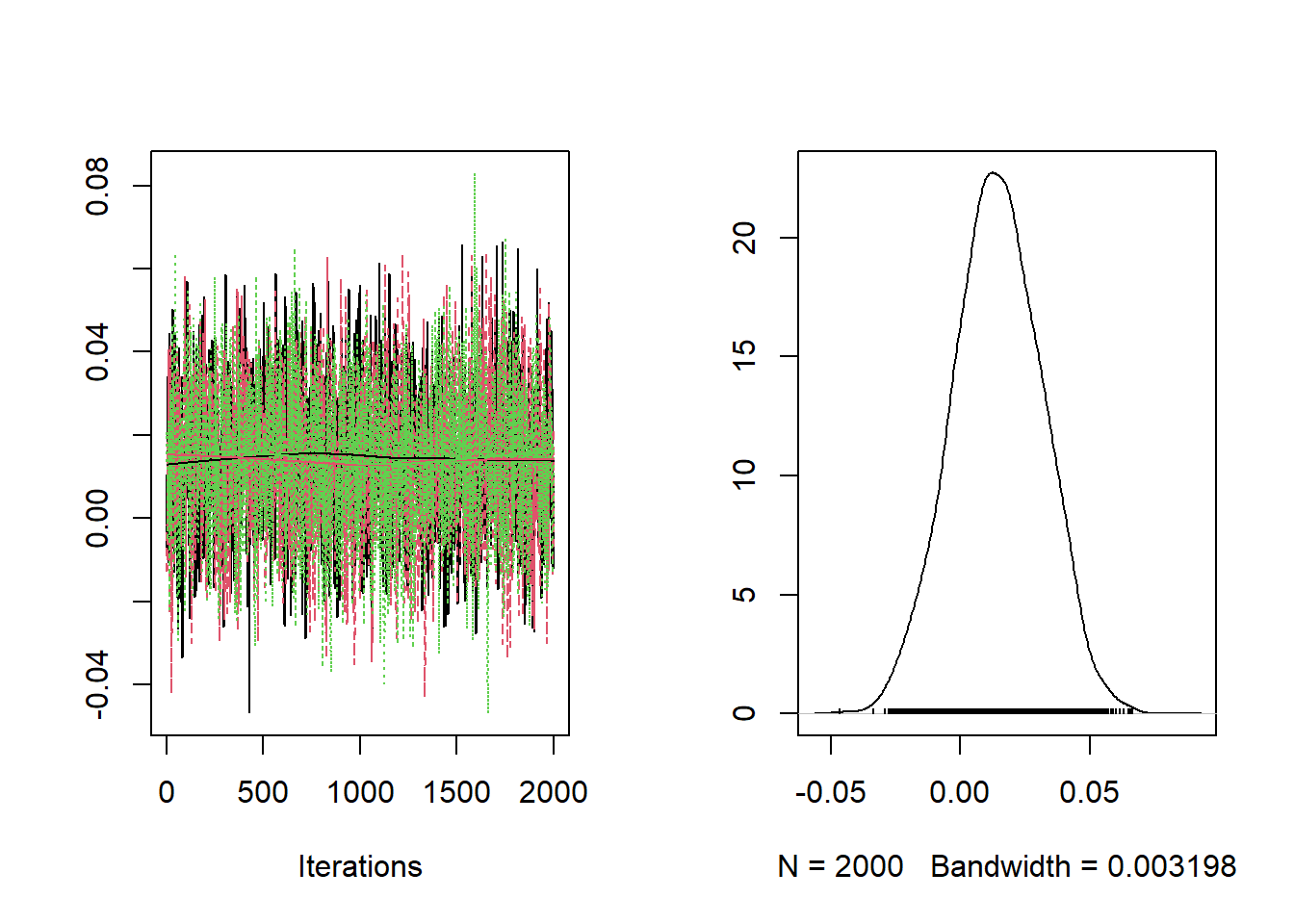
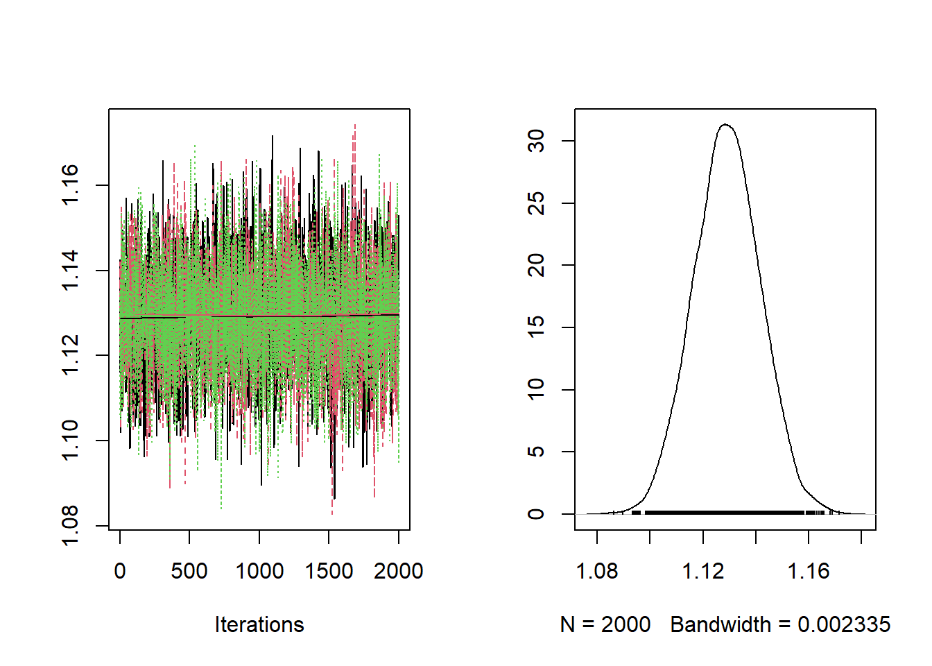
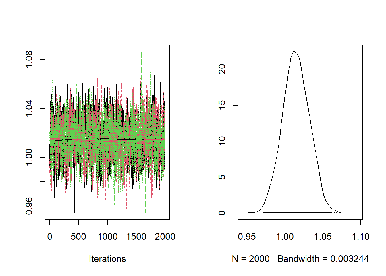
Checking the trace plots and posterior summaries for each of the parameters.
##
## Iterations = 1:2000
## Thinning interval = 1
## Number of chains = 3
## Sample size per chain = 2000
##
## 1. Empirical mean and standard deviation for each variable,
##    plus standard error of the mean:
##
##       Mean      SD  Naive SE Time-series SE
## base 1.129 0.01260 0.0001627      0.0001666
## RR   1.015 0.01744 0.0002251      0.0003443
##
## 2. Quantiles for each variable:
##
##        2.5%   25%   50%   75% 97.5%
## base 1.1046 1.121 1.129 1.138 1.154
## RR   0.9805 1.003 1.014 1.026 1.048
The baseline relative risk is estimated at 1.105 with limits of the 95% posterior credible interval equal to 1.12 and 1.154.
Stan
We now run the same example in Stan.
Load stan package with options
data {
  int<lower=0> N;
  vector[N] E; // expected cases?
  vector[N] X1; // what are these covariates?
  vector[N] X2;
  int Y[N] ;
}

parameters {
  real beta0;
  real beta1;
  real beta2;
}
transformed parameters{
  real base = exp(beta0);
  real RR = exp(beta1);
}

model {
  vector[N] mu;

  for(i in 1:N){
    mu[i] = log(E[i])+ beta0 + beta1*X1[i] + beta2*X2[i];
    Y[i] ~ poisson_log(mu[i]);
  }

  beta0 ~ normal(0 , 100);
  beta1 ~ normal(0 , 100);
  beta2 ~ normal(0 , 100);

}
data <- read.csv("data/DataExample53.csv", sep = ",")
stan_data <- list(
N = nrow(data),
E = data$exp_lungc65pls,
X1 = as.vector(scale(data$k3)),
X2 = as.vector(scale(data$k2)),
Y = data$lungc65pls
)
Example6_3_Stan <- stan(
file = "functions/Example6_3.stan",
data = stan_data,
warmup = 5000,
iter = 10000,
chains = 3,
include = TRUE
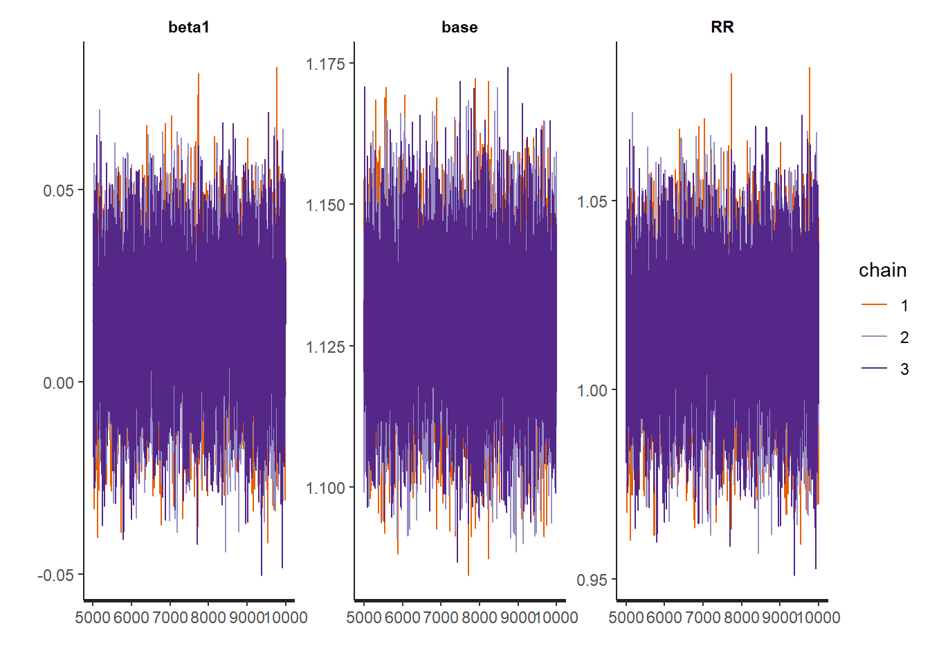
)Checking the traceplots and posterior summaries of the parameters.
##          mean      se_mean         sd      2.5%      25%      50%      75%
## RR   1.014958 0.0002226978 0.01751280 0.9808189 1.003024 1.015022 1.026792
## base 1.128715 0.0001341104 0.01258458 1.1044455 1.120106 1.128723 1.137275
##         97.5%    n_eff      Rhat
## RR   1.049442 6184.139 1.0000989
## base 1.153651 8805.473 0.9998812